Transverse Hinge Axis

Home

Scientific project

Social project

Our story

Scientific community

Book index

Our network

Frisardi Masticationpedia Network

Fontana Masticationpedia Network

Ed. Lab

Donate

Contact

Change language

[[|German]]

[[|Spanish]]

[[|French]]

[[|Italian]]

Transverse Hinge Axis

 

Article by  Gianni Frisardi · Flavio Frisardi

 

Scientific Philosophy and Clinical Implications

In the previous chapter, "Jaw_movements_analysis._Part_1:_Electrognathographic_Replicator", the disconnection between clinicians and the bioengineering foundations of diagnostic tools such as kinematic replicators was highlighted. This disconnect is particularly evident with outdated instruments like the Sirognathograph and the Kinesiograph K7, common clinical tools that, despite widespread use, fail to faithfully reproduce the three-dimensional movements of the mandible. These instruments have a significant limitation: they lose three angular degrees of freedom, two of which could theoretically be recovered, while one, related to the $Y$ axis, remains undefinable. This poses a broader problem, namely the risk that technological innovation, driven by industrial cycles, creates tools that do not fully reflect the complexity of biophysical reality. It would therefore be desirable for professionals to collaborate with research centers to critically evaluate these devices before their use. Adopting technology solely based on the manufacturer's reputation has led to the phenomenon of the Research Diagnostic Criteria "RDC," which was created to eliminate methods and tools with low clinical validity. This chapter will explore the concept of the "Hinge Axis" $HA$, an extensively studied and debated topic that continues to raise questions regarding its actual clinical and diagnostic usefulness. The determination of the hinge axis was traditionally performed using methods initially described by McCollum, and subsequently perfected over the years. This method, known as the "kinematic pantographic method," uses the length of the mandibular opening segment as a key parameter, providing generally acceptable accuracy, though not free from errors.

With the development of electronic recording systems such as the SICAT JMT and the Zebris JMA, precision in determining the hinge axis has improved, reducing adjustment times and potentially increasing accuracy to $\pm 1$ ${\textstyle mm}$. However, the question remains whether the initial opening movement of the mandible is purely rotational or combined with translation.

«Scientific Philosophy or speculative trend?»
(...perhaps reality eludes our limited bioengineering competence, and statistical models are incapable of revealing instrumental limitations.)

Occlusal Clutch and Cuspal Errors

We will first focus on the scientific philosophy behind the concept of the transverse hinge axis, commonly projected onto a sagittal plane and labeled '$_{t}HA$'. The main goal is to establish whether this concept should continue to be used as a reference in masticatory rehabilitation practices, or if it should be revised or abandoned to avoid clinical practice errors, as asserted by the RDC. A key aspect to explore is the phenomenon of rototranslation, a fundamental element of mandibular kinematics. This complex movement will be analyzed through practical examples and explanatory figures, demonstrating how tools such as the paraocclusal clutch can avoid the incorporation of significant errors in the registration of mandibular movements and occlusal dynamics. Precision in determining mandibular movements is crucial not only to ensure the accuracy of rehabilitative treatments but also to avoid discrepancies in prosthetic restorations. Small variations, if not adequately considered, can compromise the recording of movements and, consequently, alter the functionality of rehabilitation. A method of recording condylar tracings will be illustrated using the clutching with a paraocclusal clutch, which has the advantage of not altering the vertical relationship between dental arches. This method will be compared with the mounting of an occlusal clutch to highlight the differences between the two approaches.

• Figure 1: To precisely determine a geometric center of rotation or, more accurately, of rototranslation, it is necessary to connect a writing stylus to a frame attached to the mandible. This system follows mandibular movements during chewing cycles, tracing a path on a perpendicular plate fixed to a rigid support on the skull. This connection is generally made through the cementation of an intraoral clutch, called an occlusal clutch.

• Figure 2: The figure shows a typical paraocclusal clutch, which does not interfere with the maxillary occlusal surface, allowing for maximum intercuspation without causing a vertical lift or a rototranslation of the condylar joint.

• Figure 3: The figure depicts the tracing generated from mandibular opening and closing movements and left mediotrusion using a paraocclusal clutch. Some key points are as follows:

First point: A red point located on a horizontal line representing the 'Axis-Orbital' plane. This point corresponds to the guided hinge axis and is labeled as $P_{c}$ (Paraocclusal clutch), with an orbital reference point indicated as $O_{p}$ (Orbital point). The red point approximately represents the $_{t}HA$ axis.

Second point: Another point, located about 2 mm in protrusion, corresponds to a mandibular opening of about 4 mm, measured at the incisors, and is due to the use of an occlusal clutch between the arches. This point is labeled as $O_{c}$ (Occlusal Clutch).

Third point: At the end of the mandibular opening trace is point $H$.

From these strategic points, important considerations can be made regarding the determination of the hinge axis using a paraocclusal or occlusal clutch. In Figure 3, a line has been drawn from $P_{c}$ to $H$, representing the angle of the Articular Eminence, calculated with Geogebra, yielding a value of $41.69^{\circ }$ compared to an angle of $50.20^{\circ }$ for the line drawn between $O_{c}$ and $H$.

The choice of using $P_{c}$ or $O_{c}$ can generate a significant error, with an angular variation of $8.51^{\circ }$, which can reach up to $10^{\circ }$, as indicated by Oliver Schierz et al. This error is transferred to the prosthetic phase, generating a spatial discrepancy in the cuspal position.

• 

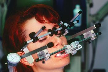
  Figure 1: Axiography performed through occlusal clutch

• 

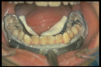
  Figure 2: Paraocclusal clutch

• 

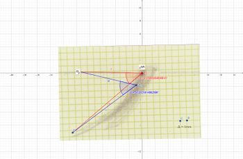
  Figure 3:

Localization Error $_{t}HA$ from Chord $s$ and Sagitta $h$

To achieve an accurate determination of the mandibular rotation axis, the widest possible opening rotation is chosen. The literature describes mouth opening values between 7 and 18 mm, during which an almost pure rotation occurs before further translational movement begins. While it is debatable whether an opening of 15 mm truly represents pure rotation, this value can be considered the upper limit for optimal hinge axis detection. The radius of movement, particularly of the incisal point, can be calculated using the average Bonwill triangle, which measures approximately 90.7 mm. With this radius and an opening of 15 mm, the opening angle corresponds to about 9.5 degrees. Simulations and calculations were implemented in Python, and the results were geometrically visualized in Geogebra for a spatial representation and better understanding of the phenomenon. Any recorded opening movement from an appropriate measuring device will describe a path that lies on a segment of a circular arc. The task is to determine the radius of this movement or, more precisely, the location of the center of rotation.

In our case (Figure 4), it is possible to identify two arcs of a circle and a center of rotation corresponding to the arc generated by a mandibular opening with forced retrusion. The arc where a presumably precise center of pure rotation, or rather "relatively pure," is found is generated by keeping the mandible forcibly retruded so that it rotates around the temporomandibular ligament, thereby minimizing the translation of the temporomandibular joint (TMJ). This maneuver allows for the distinction of the rototranslational pattern that occurs in the absence of forced retrusion and/or manual guidance (represented by the underlying arc). In Figure 4, the traces differ significantly because the second (lower) one incorporates both rotation and translation simultaneously.

When measuring something, such as the distance between two points on a circle, the measurement is not always perfect; small errors or "noise" can affect the result. We want to explore how these small errors can compromise the estimate of a measurement that should be precise. Figure 5 and the accompanying Python script enhance the representation. This type of analysis is useful because it allows us to assess the reliability of our measurements in real-life situations, where there are always small inaccuracies. It is particularly relevant in fields such as biomechanics or engineering, where measurements need to be highly accurate.

Theoretically, the radius can be recalculated from the circular-like opening movement using the chord $s$ and the sagitta (height) $h$ (Figure 5). From these values, the radius of the circumference inscribed in the pure rotation arc, physically constructed on the plate and labeled as $0$, can be calculated and verified for discrepancies as $0_{1}$ using Geogebra.

From the data obtained with Geogebra, it is possible to construct, first, the radius of $0_{1}$ (forced opening in retrusion, presumably rotational), and, of course, determine the centers of rotation. The mathematical formalism to achieve this is as follows:

$r_{calc}={\frac {4h+s^{2}}{8h}}$

By substituting $s$ and $h$ with the values obtained from Geogebra, we obtained a maximal error in the localization of Center $0_{1}$ of approximately $\cong 4.95$ ${\textstyle mm}$ at a percentile of $72\%$ (see Figure 6). Measuring the distance with Geogebra between centers $0_{1}$ and $0$, it results in $\Delta =1.73$ ${\textstyle mm}$, which corresponds to an error of 30% compared to the maximal value of $\cong 4.95$. This means that visually and manually locating the center of rotation can result in an error of about $\cong 1.73$ ${\textstyle mm}$ compared to a mathematical calculation on the mandibular opening and closing trace.

• 

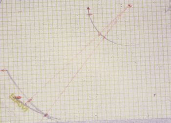
  Figura 4: Tracciati assiografica di apertura e chiusura della bocca in retrusione forzata ( arco di cerchio a sinistra della finestra) e guidata ( sottostante). In seguito verranno descritti più dettagliatamente i tracciati.

• 

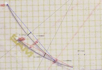
  Figura 5: Determinazione dei parametri $s$ ed $h$ necessari per generare un centro di rotazione.

• 

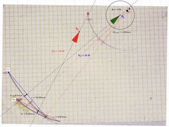
  Figura 6: Discrepanza tra asse cerniera generato visivamente dall'operatore e matematicamente in Geogebra.

Mathematical Formalism: Localization Error of HA from Chord $s$ and Sagitta $h$

The script simulates the effect of noise on the measurement of the distance between a fixed point and a hinge axis (HA). A distribution of errors caused by noise added to the data is generated, and the 72nd percentile of these errors is analyzed.

The radius ($r$) is the radius of the circle on which the initial point lies, given by $r=26.30$ mm. The arc length $s$ is the length of the arc on which the point moves, equal to $s=12.02$ mm. The angle $\alpha$ is the angle corresponding to the arc, in radians, calculated as:

$\alpha ={\frac {s}{r}}$

$r_{\text{var}}$: This is the distance of the starting point from the hinge axis, equal to $r_{\text{var}}=26.30$ mm. To calculate the start and end points, we proceed by calculating the point $p_{\text{start}}$, located at a distance $r_{\text{var}}$ along the $x$-axis:

$p_{\text{start}}={\begin{pmatrix}r_{\text{var}}\ 0\end{pmatrix}}$

The terminal point $p_{\text{end}}$ is defined as the final point after the rotation of an angle $\alpha$, calculated as:

$p_{\text{end}}={\begin{pmatrix}r_{\text{var}}\cos(\alpha )\ r_{\text{var}}\sin(\alpha )\end{pmatrix}}$

The length of the chord $s_{\text{ref}}$ that connects the initial and final points is given by:

$s_{\text{ref}}={\sqrt {(p_{{\text{end}},x}-p_{{\text{start}},x})^{2}+(p_{{\text{end}},y}-p_{{\text{start}},y})^{2}}}$

The height of the arc (sagitta) $h_{\text{ref}}$ is calculated as:

$h_{\text{ref}}={\frac {s_{\text{ref}}}{2}}\tan \left({\frac {\alpha }{4}}\right)$

At this point, Gaussian-distributed noise with a standard deviation of 0.01 mm is generated. The noise is added to the start and end points as follows:

$pn_{\text{start}}=p_{\text{start}}+noise_{\text{start}}$

$pn_{\text{end}}=p_{\text{end}}+noise_{\text{end}}$

This extends or shortens the chord $s$ as follows:

${\sqrt {(pn_{end,x}-pn_{start,x})^{2}+(pn_{end,y}-pn_{start,y})^{2}}}$

While the noise on the sagitta $h_{\text{noise}}$ is calculated as:

$h_{\text{noise}}=h_{\text{ref}}+{\text{noise}}$

Once the errors for the chord $s$ and the sagitta $h$ are calculated, we can compute the noisy radius $r_{\text{noise}}$ by reusing the formula:

$r_{\text{noise}}={\frac {4h_{\text{noise}}^{2}+s^{2}}{8h_{\text{noise}}}}$

The difference between the radius calculated with noise and the original distance $r_{\text{var}}$ is given by:

$\delta r_{\text{noise}}=\left|r_{\text{noise}}-r_{\text{var}}\right|$

At the 72nd percentile of the measurement error, this represents the value below which 72% of the observed errors fall.

Script Python: Errore localizzazione HA da corda $s$ e sagitta $h$

import numpy as np
import matplotlib.pyplot as plt

# Constants
r = 90.7  # Radius in mm
s = 12.02  # Length of Arc in mm
alpha = s / r  # Angle in radians
r_var = 26.33  # Distance from the hinge axis in mm

# Calculate start and end points
p_start = np.array([r_var, 0])
p_end = np.array([r_var * np.cos(alpha), r_var * np.sin(alpha)])

# Calculate reference values
s_ref = np.sqrt((p_end[0] - p_start[0])**2 + (p_end[1] - p_start[1])**2)
h_ref = s_ref / 2 * np.tan(alpha / 4)
scale_noise = 0.01  # Reduced noise in mm
samples = 1000  # number of Gaussian samples
noise = scale_noise * np.random.randn(5, samples)

# Add noise to points
pn_start = np.array([p_start[0] + noise[0, :], p_start[1] + noise[1, :]])
pn_end = np.array([p_end[0] + noise[2, :], p_end[1] + noise[3, :]])

# Calculate length of the chord (s) and sagitta (height) (h_noise)
s = np.sqrt((pn_end[0, :] - pn_start[0, :])**2 + (pn_end[1, :] - pn_start[1, :])**2)
h_noise = h_ref + noise[4, :]
r_noise = (4 * h_noise**2 + s**2) / (8 * h_noise)
delta_r_noise = np.abs(r_noise - r_var)

# Calculate the 72nd quantile of the error
error_quantile_reduced_noise = np.quantile(delta_r_noise, 0.72)
print(f'Errore (72° percentile) con rumore ridotto: {error_quantile_reduced_noise:.2f} mm')

# Optional: Plot the distribution of errors
plt.hist(delta_r_noise, bins=30, edgecolor='k', alpha=0.7)
plt.axvline(error_quantile_reduced_noise, color='r', linestyle='dashed', linewidth=1)
plt.title('Distribuzione degli errori di misurazione')
plt.xlabel('Errore (mm)')
plt.ylabel('Frequenza')
plt.show()

Trace Resolution and Point Fitting

The approximate calculation presented in the previous section considers only the initial and final points of a movement that follows an arc of a circle, along with the segment distance $h$ (or, to remain consistent with other calculations, three points on the circumference). Modern measuring devices can record the positions of mandibular movement at very short time intervals, but even in this case, not everything is perfect. The problem shifts to the sampling capabilities of the phenomenon and the recording channels (topics that will be addressed in due course). Therefore, not only the initial and final points are known, but also many other points along the trace can be measured. It is assumed that this additional information can improve the accuracy of determining the hinge axis. Under ideal conditions, all these points should lie on a segment of a circle around the hinge axis. By fitting a circle to these points, the hinge axis can be determined with precision. However, the imprecision of each measurement introduces uncertainty at each point (Fig. 7). This "noise" affects the detection of the hinge axis.

The best algorithms for reconstructing rotational movement are those that use a least-squares optimization approach to fit a circle. The most effective methods are the Taubin fitting or Pratt fitting methods, both available in MATLAB. In our case, we used the Levenberg-Marquardt method.

Levenberg-Marquardt Method: This method is extremely versatile and can be applied to a wide range of non-linear fitting problems, not only for fitting circles but also other curves or surfaces. It is known for its ability to converge even when the initial estimate is not particularly close to the optimal solution. This method is a compromise between the gradient method and the Gauss-Newton method, balancing efficiency and stability. The Levenberg-Marquardt method is well-supported by many numerical optimization libraries, such as SciPy in Python, making it a practical and accessible choice for most users. Its implementation is relatively simple and well-documented, making it suitable for anyone wishing to perform curve or surface fitting quickly. Since the problem of fitting a circle is non-linear (due to the quadratic dependence of the coordinates on the circle's center), the Levenberg-Marquardt method is well-equipped to handle these complexities.

Taubin Method: The Taubin method, on the other hand, is particularly recommended when a circle fitting that is less sensitive to noise and measurement errors is desired. This method minimizes the orthogonal error, which often better represents real errors in experimentally collected data. If the priority were to robustly minimize the error, regardless of the direction of fitting, the Taubin method might be more appropriate.

The choice between Levenberg-Marquardt and Taubin depends on the specific needs of the problem and the characteristics of the data. For general non-linear fitting problems with good initial estimates and the need for a quick and practical solution, Levenberg-Marquardt is a solid choice. However, for more specialized applications, such as precise circle or conic fitting, the Taubin method may offer advantages in terms of accuracy and robustness.

In conclusion, the simulation showed that the fitting method used was able to estimate both the center and radius of the circle with good accuracy, despite the presence of noise in the data. The overall error is low, indicating that the effect of noise on the final result was minimal. An error of $\cong 0.63$ ${\textstyle mm}$ is rather small, which implies that the fitting was accurate despite the noise introduced into the data. This error represents the deviation of the calculated circle's center from the true center.

Figure 7 illustrates the dependency of the hinge axis determination on the distance of the measurement position from the center of rotation. It also highlights that a measurement close to the TMJ (with a small radius) does not offer greater accuracy with the circle fitting method compared to a measurement taken further from the TMJ or closer to the jaw (e.g., at the incisal point). On the contrary, radii smaller than $20$ ${\textstyle mm}$ significantly increase the imprecision in determining the hinge axis. This result is positive in a clinical context, as it indicates that, even in the presence of noise (as can happen in real measurements), it is possible to accurately estimate the $_{t}HA$ and the associated radius, which are crucial for patient diagnosis and rehabilitative treatment.

• 

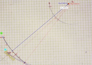
  Figura 7:

Mathematical Formalism: Fitting Error

To illustrate the concept of error due to noise in determining the points of the curve, the preliminary mathematical steps are as follows (refer to Figure 7, represented in Geogebra).

The script starts by defining the original circle center with the coordinates:

$O_{HA}={\begin{pmatrix}11.55\ 61.14\end{pmatrix}}$

This center represents the central point around which a circle will be constructed.

The radius of the circle is set to $r=26.38$ mm. This value represents the distance from the center to the points on the edge of the circle. Using the center and radius, 10 points are uniformly distributed along the circumference of the circle. The angles $\theta$ used to position the points are distributed from $0$ to $2\pi$. For each angle, the coordinates of the points are calculated using the parametric equations of the circle:

$x=x_{c}+r\cdot \cos(\theta )$

$y=y_{c}+r\cdot \sin(\theta )$

A function called add_noise_to_points is used to add noise to the generated points. The noise is generated from a normal (or Gaussian) distribution with a mean of zero and a standard deviation of $0.1$ units. This step simulates the measurement errors that may occur in practice. The points disturbed by noise are stored in the noisy_points variable.

The function residuals is defined to calculate the residuals, that is, the difference between the distance of each noisy point from the estimated center and the estimated radius. This function is essential for optimization since the circle fitting aims to minimize these residuals:

$R_{i}={\sqrt {(x_{i}-x_{c})^{2}+(y_{i}-y_{c})^{2}}}-r$

where $R_{i}$ is the residual for the $i$-th point.

An initial estimate of the noisy circle's center is made by calculating the mean of the noisy points' coordinates:

$x_{m}={\frac {1}{n}}\sum _{i=1}^{n}x_{i}$, $y_{m}={\frac {1}{n}}\sum _{i=1}^{n}y_{i}$

This average is used as a starting point for the fitting.

Initial Radius

The initial radius is estimated as the mean distance between each noisy point and the estimated center:

$r_{m}={\frac {1}{n}}\sum _{i=1}^{n}{\sqrt {(x_{i}-x_{m})^{2}+(y_{i}-y_{m})^{2}}}$

This approximated value is used as the initial radius for the optimization.

Circle Fitting with Levenberg-Marquardt Method

• Fitting Optimization:

The least_squares function from the SciPy library is used to perform the circle fitting. This method minimizes the residuals calculated earlier, aiming to find the optimal values for the center coordinates $(x_{c},y_{c})$ and the radius $r$. The optimization results are returned as the calculated center $(x_{c},y_{c})$ and the radius $r$.

Error Calculation

• Error between Centers:

The distance between the calculated center and the original center is computed. This distance represents the localization error, indicating how far the calculated center deviates from the true center due to noise:

${\text{error}}={\sqrt {(x_{c}-x_{\text{original}})^{2}+(y_{c}-y_{\text{original}})^{2}}}$

The error is then converted into millimeters if the original units were in centimeters, for greater interpretative precision.

Script Python: Errore di fitting

import numpy as np
from scipy.optimize import least_squares
import matplotlib.pyplot as plt

# Original data provided
original_center = np.array([11.56, 61.21])
radius = 26.38
angles = np.linspace(0, 2 * np.pi, 10)
points = np.array([
    original_center + radius * np.array([np.cos(angle), np.sin(angle)])
    for angle in angles
])

# Function to add noise to the points
def add_noise_to_points(points, noise_level):
    noisy_points = points + np.random.normal(0, noise_level, points.shape)
    return noisy_points

# Add noise to the points
noise_level = 0.1  # Reduced noise level
noisy_points = add_noise_to_points(points, noise_level)

# Residual function for non-linear fitting
def residuals(c, points):
    xc, yc, r = c
    Ri = np.sqrt((points[:, 0] - xc)**2 + (points[:, 1] - yc)**2)
    return Ri - r

# Calculate the center and radius using noisy points
x_m = np.mean(noisy_points[:, 0])
y_m = np.mean(noisy_points[:, 1])
r_m = np.mean(np.sqrt((noisy_points[:, 0] - x_m)**2 + (noisy_points[:, 1] - y_m)**2))
initial_guess = [x_m, y_m, r_m]

# Fitting the circle using the Levenberg-Marquardt method
result = least_squares(residuals, initial_guess, args=(noisy_points,))
xc, yc, r = result.x

calculated_center = np.array([xc, yc])

# Calculate the error between the centers
error = np.linalg.norm(calculated_center - original_center)
error_mm = error * 10  # Convert to millimeters (assuming the points might be in centimeters)

# Verify the calculated center
print(f'Calculated Center: {calculated_center}')
print(f'Radius: {r:.4f}')
print(f'Error: {error_mm:.4f} mm')

# Visualization of the fitted circle
theta = np.linspace(0, 2 * np.pi, 100)
x_fit = calculated_center[0] + r * np.cos(theta)
y_fit = calculated_center[1] + r * np.sin(theta)

plt.figure(figsize=(8, 8))
plt.scatter(points[:, 0], points[:, 1], color='b', label='Original Points')
plt.scatter(noisy_points[:, 0], noisy_points[:, 1], color='r', label='Noisy Points')
plt.scatter(original_center[0], original_center[1], color='r', marker='x', s=100, label='Original Center')
plt.plot(x_fit, y_fit, 'g--', label='Fitted Circle')
plt.scatter(calculated_center[0], calculated_center[1], color='g', label='Calculated Center')
plt.xlabel('X')
plt.ylabel('Y')
plt.legend()
plt.title('Circle Fitting with Noisy Points')
plt.grid(True)
plt.show()

Occlusal Distortions

In dentistry and gnathology, a precise understanding of mandibular movements is essential for designing accurate dental prostheses. One of the key concepts in this field is $_{t}HA$, which represents the axis around which the mandible rotates during the first millimeters of mouth opening. The correct localization of $_{t}HA$ is crucial for achieving natural mandibular movement and proper dental occlusion. An inaccurate localization of $_{t}HA$ can lead to significant errors in the final position of the dental cusps. Cusps are the points of the teeth that interlock between the upper and lower teeth during mastication. If $_{t}HA$ is not correctly localized, especially in the presence of inclined cusps, the error may manifest as a discrepancy between the predicted and actual position of the cusps. This can compromise the effectiveness of dental treatments and lead to malocclusion or discomfort for the patient.

The objective of this simulation is to explore and quantify how the error in localizing $_{t}HA$ affects the position of the dental cusps, considering two specific scenarios:

• Mandibular Opening of $0$ ${\textstyle mm}$: This parameter represents the centric recording model without wax interposed between the arches. With a mandibular opening of $0$ ${\textstyle mm}$, the cuspal error is theoretically zero if the cusps were flat. However, if the cusps are inclined, the error may not be zero due to the inclination itself. *Mandibular Opening of $3$ ${\textstyle mm}$: This parameter represents the centric recording model with wax interposed between the arches, generating a mandibular opening of $3$ ${\textstyle mm}$. In this condition, even a small error in the localization of $_{t}HA$ can cause a significant cuspal error, exacerbated by the inclination of the dental cusps.

Simulation Results

To address this problem, we use mathematical models and computer simulations to calculate how an error in the localization of $_{t}HA$ translates into errors in the final positions of the dental cusps. We use various magnitudes of $_{t}HA$ localization error (up to $10$ ${\textstyle mm}$) and analyze the effect of these discrepancies both with centric recordings without wax and with the mouth closed ($0$ ${\textstyle mm}$) as well as with a slight mouth opening ($3$ ${\textstyle mm}$). In addition, we consider the inclination of the dental cusps, simulating errors on inclined cusps of $0^{\circ }$ and $5^{\circ }$ to make the model more realistic and applicable to actual clinical conditions. This approach allows us to better understand how localization errors affect the final result and provides valuable insights for improving precision in dental practices.

In essence, with an opening of $0$ ${\textstyle mm}$ in centric recordings without wax and non-inclined cusps ($0^{\circ }$), and with a $_{t}HA$ error of $10$ ${\textstyle mm}$ (10 steps from $0$ ${\textstyle mm}$ to $10$ ${\textstyle mm}$), the cuspal error is $0$ ${\textstyle mm}$. With a mandibular opening of $3$ ${\textstyle mm}$ and flat dental cusps ($0^{\circ }$), the cuspal error ranges from $0$ ${\textstyle mm}$ in a situation of exact $_{t}HA$ localization to $1$ ${\textstyle mm}$ with a localization error of $10$ ${\textstyle mm}$. However, even if we were to perform a centric recording without wax with a mandibular opening of $0$ ${\textstyle mm}$, with dental cusps inclined by just $5^{\circ }$, this condition introduces a vertical cuspal error due to the projection of the $_{t}HA$ localization error along the inclination of the cusps. In this case, the error ranges from $0$ ${\textstyle mm}$ in an exact localization of $_{t}HA$ to $0.87$ ${\textstyle mm}$ with a localization error of $10$ ${\textstyle mm}$.

Script Pyhton: Errore Cuspidale con Apertura a 0 mm e Cuspidi Piatte'

import numpy as np
import matplotlib.pyplot as plt

# Definition of the original data
original_center = np.array([11.56, 61.21])  # Original center of the circle
r = 26.38  # Radius of the original circle
theta = np.linspace(0, 2 * np.pi, 10)  # 10 points along the circumference

# Generation of original points on the circumference
points = np.array([
    original_center + r * np.array([np.cos(angle), np.sin(angle)])
    for angle in theta
])

# Definition of the radius for the position of dental cusps
cusp_radius = 75.0  # Distance of the cusp from the center of rotation

# Generation of the positions of the original dental cusps
cusp_positions = np.array([
    original_center + cusp_radius * np.array([np.cos(angle), np.sin(angle)])
    for angle in theta
])

# Simulation of the errors Δ
errors = np.linspace(0, 10, 10)  # Errors Δ from 0 to 10 mm, 10 steps
max_differences_zero_apertura = []

# Cusp error for mandibular opening at 0 mm is zero
for delta in errors:
    max_differences_zero_apertura.append(0)  # Cusp error is zero

plt.plot(errors, max_differences_zero_apertura, 'ro-', label='Opening 0 mm (Mouth closed)')
plt.xlabel('Error Δ (mm) in HA localization')
plt.ylabel('Max Difference in Cusp Positions (mm)')
plt.title('Cusp Error with 0 mm Opening and Flat Cusps')
plt.grid(True)
plt.legend()
plt.show()

Script Pyhton: Errore Cuspidale con Apertura a 3 mm e Cuspidi Piatte

import numpy as np
import matplotlib.pyplot as plt

# Definition of the original data
original_center = np.array([11.56, 61.21])  # Original center of the circle
r = 26.38  # Radius of the original circle
theta = np.linspace(0, 2 * np.pi, 10)  # 10 points along the circumference

# Generation of original points on the circumference
points = np.array([
    original_center + r * np.array([np.cos(angle), np.sin(angle)])
    for angle in theta
])

# Definition of the radius for the position of dental cusps
cusp_radius = 75.0  # Distance of the cusp from the center of rotation

# Generation of the positions of the original dental cusps
cusp_positions = np.array([
    original_center + cusp_radius * np.array([np.cos(angle), np.sin(angle)])
    for angle in theta
])

# Simulation of the errors Δ
errors = np.linspace(0, 10, 10)  # Errors Δ from 0 to 10 mm, 10 steps
max_differences_apertura_3mm = []

# Calculation of the cusp error for a mandibular opening of 3 mm
for delta in errors:
    new_center = original_center + np.array([delta, 0])  # Shift along the x-axis
    
    # Calculate the new positions of the dental cusps with error Δ
    new_cusp_positions = np.array([
        new_center + cusp_radius * np.array([np.cos(angle), np.sin(angle)])
        for angle in theta
    ])
    
    # Calculate the spatial differences between the original and calculated positions
    differences = np.linalg.norm(cusp_positions - new_cusp_positions, axis=1)
    max_difference = np.max(differences) * (3 / 30)  # Scaling the error for a 3 mm opening out of 18 mm maximum
    max_differences_apertura_3mm.append(max_difference)
    
    print(f"Error Δ = {delta:.1f} mm: Max Difference in Cusp Positions (3 mm opening) = {max_difference:.2f} mm")

plt.plot(errors, max_differences_apertura_3mm, 'bo-', label='Opening 3 mm')
plt.xlabel('Error Δ (mm) in HA localization')
plt.ylabel('Max Difference in Cusp Positions (mm)')
plt.title('Cusp Error with 3 mm Opening and Flat Cusps')
plt.grid(True)
plt.legend()
plt.show()

Script Python: Effetto degli Errori di Localizzazione del Centro di Rotazione con on Apertura a 0 mm e Cuspidi Inclinate $5^{\circ }$

import numpy as np
import matplotlib.pyplot as plt

# Definition of the original data
original_center = np.array([11.56, 61.21])  # Original center of the circle
r = 26.38  # Radius of the original circle
theta = np.linspace(0, 2 * np.pi, 10)  # 10 points along the circumference

# Generation of original points on the circumference
points = np.array([
    original_center + r * np.array([np.cos(angle), np.sin(angle)])
    for angle in theta
])

# Definition of the radius for the position of dental cusps
cusp_radius = 75.0  # Distance of the cusp from the center of rotation

# Generation of the positions of the original dental cusps
cusp_positions = np.array([
    original_center + cusp_radius * np.array([np.cos(angle), np.sin(angle)])
    for angle in theta
])

# Simulation of the errors Δ
errors = np.linspace(0, 10, 10)  # Errors Δ from 0 to 10 mm, 10 steps
max_differences_inclined_cusp = []

# Definition of the angle of the dental cusps (in degrees)
cusp_angle_deg = 5  
cusp_angle_rad = np.deg2rad(cusp_angle_deg)  # Conversion to radians

# Calculation of cusp error for mandibular opening at 0 mm with inclined cusps
for delta in errors:
    # Calculation of vertical error due to cusp inclination
    vertical_error_due_to_inclination = delta * np.tan(cusp_angle_rad)
    
    # Save the maximum error in this specific case
    max_differences_inclined_cusp.append(vertical_error_due_to_inclination)
    
    print(f"Error Δ = {delta:.1f} mm: Max Difference in Cusp Positions with inclined cusps = {vertical_error_due_to_inclination:.2f} mm")

plt.plot(errors, max_differences_inclined_cusp, 'ro-', label=f'Inclined Cusps ({cusp_angle_deg}°)')
plt.xlabel('Error Δ (mm) in HA localization')
plt.ylabel('Max Difference in Cusp Positions (mm)')
plt.title(f'Effect of Rotation Center Localization Errors with Inclined Cusps ({cusp_angle_deg}°)')
plt.grid(True)
plt.legend()
plt.show()

Discussion

In the context of this chapter, one of the deepest tensions characterizing modern gnathology has emerged: the importance of the '6 degrees of freedom' in ensuring optimal masticatory efficiency and the growing tendency of the 'RDC' to exclude mandibular kinematic tools from clinical practice. While the stated goal of the RDC is to improve diagnostic effectiveness by eliminating methodologies with low clinical validity, the assertion of removing kinematic replicators from dental practice appears controversial. This is because mandibular kinematics is a fundamental element in understanding not only mandibular movements but also the masticatory forces that influence the duration and effectiveness of mastication.

Masticatory efficiency, for example, does not depend solely on the strength applied by the muscles or the robustness of the dental structure but also on the mandible's ability to move through its '6 degrees of freedom', allowing the proper functioning of the teeth in cutting and grinding food. Each degree of freedom—three translations (along the $x,y,z$ axes) and three rotations (around the same axes)—contributes to the complex interaction between dental surfaces and muscular forces, which is in turn influenced by the normal and tangential forces generated by occlusal contact. In the case of molar teeth, the natural inclination of the cusps helps reduce the dispersion of metabolic energy during the cutting process, maximizing masticatory efficiency. Without this natural inclination, mastication would become less efficient, leading to higher energy expenditure and increased muscular and joint load. As shown in previous simulations, an incorrect localization of the transverse hinge axis ($_{t}HA$) can significantly affect the precision of the cusps and, therefore, the proper alignment of the teeth during occlusal contact.

The RDC's argument is based on the assumption that mandibular kinematic tools, such as gnathological replicators and pantographs, do not make a significant contribution to improving prosthetic rehabilitations. However, this statement seems debatable in light of biomechanical and clinical evidence. In particular, diagnostic tools that allow the analysis of mandibular movements in three dimensions, such as the SICAT JMT and Zebris JMA systems, have shown that mandibular movement is not purely rotational but involves a component of 'rototranslation'. This combination of movement is crucial for faithfully replicating mandibular function, especially in patients with complex occlusal issues. Mandibular kinematics provides a deeper understanding not only of the occlusal contact angle but also of how muscular forces and dental resistances balance during the masticatory cycle. The RDC tends to argue that three-dimensional analysis tools are too costly, complex, and not useful in daily practice. However, the data presented in this chapter indicate the opposite: the use of such tools can prevent significant errors in prosthetic rehabilitation and improve therapeutic effectiveness.

In the simulations presented, we demonstrated that even a small error in the localization of $_{t}HA$ can lead to significant discrepancies in the position of dental cusps. Specifically, with a mandibular opening of just 3 mm and cusps inclined at $5^{\circ }$, an error in the localization of the axis of 10 mm can cause a vertical cuspal error of nearly 1 mm. While this may seem minimal, it is a discrepancy sufficient to compromise the prosthetic's effectiveness and cause discomfort for the patient.

On the other hand, with a mandibular opening of 0 mm (mouth closed), the cuspal error is theoretically zero only in the case of flat cusps ($0^{\circ }$), whereas with cusps inclined by even a few degrees, an error margin is still introduced due to the projection of the localization error onto the inclination itself. This shows that without accurate kinematic analysis, it is impossible to guarantee proper alignment of the cusps and occlusal surfaces, with significant repercussions on the patient's masticatory function.

In light of these observations, it is clear that the exclusion of kinematic tools from clinical practice, as suggested by the RDC, is not a scientifically founded choice. Kinematic tools offer a unique understanding of mandibular movements, allowing clinicians to accurately replicate mandibular motions and ensure superior prosthetic treatment. Removing such tools from clinical practice could reduce diagnostic and treatment precision, leading to an increased risk of malocclusion, temporomandibular disorders, and patient discomfort.

The data presented clearly show that determining the transverse hinge axis ($_{t}HA$) and controlling rototranslational movements are crucial for minimizing energy dispersion and optimizing masticatory efficiency. The inclination of the cusps, the proper alignment of occlusal surfaces, and the precision in localizing the axis of rotation must be treated with the utmost care to avoid errors that could compromise clinical outcomes.

In conclusion, while the RDC argues that kinematic tools are not essential for daily clinical practice, the scientific evidence presented indicates that these tools are crucial for accurate evaluation and rehabilitation of masticatory function. Eliminating these tools from clinical practice would not only reduce diagnostic accuracy but also compromise the quality of care provided to patients. It is therefore essential that professionals continue to integrate the use of advanced kinematic tools into their practice to ensure optimal prosthetic treatment and a high quality of life for patients.

«But then, is it enough to only know the dynamics of $_{t}HA$?»
(.....certainly not. The mandibular kinematic phenomenon, being a 6 degrees of freedom dynamic, requires mandatory knowledge of the vertical axis $_{a}HA$ on the axial plane and the sagittal axis $_{c}HA$ on the coronal plane. Topics we will address in the next chapters)

Bibliography & references