|
|
| (4 intermediate revisions by one other user not shown) |
| Line 1: |
Line 1: |
| {{transl}}
| |
|
| |
|
|
| |
|
| Line 29: |
Line 28: |
| {{Bookind2}} | | {{Bookind2}} |
|
| |
|
| == Abstract ==
| | {{:Store:QLMen01}} |
| We present the novel approach to mathematical modeling of information processes in biosystems. It explores the mathematical formalism and methodology of quantum theory, especially quantum measurement theory. This approach is known as ''quantum-like'' and it should be distinguished from study of genuine quantum physical processes in biosystems (quantum biophysics, quantum cognition). It is based on quantum information representation of biosystem’s state and modeling its dynamics in the framework of theory of open quantum systems. This paper starts with the non-physicist friendly presentation of quantum measurement theory, from the original von Neumann formulation to modern theory of quantum instruments. Then, latter is applied to model combinations of cognitive effects and gene regulation of glucose/lactose metabolism in Escherichia coli bacterium. The most general construction of quantum instruments is based on the scheme of indirect measurement, in that measurement apparatus plays the role of the environment for a biosystem. The biological essence of this scheme is illustrated by quantum formalization of Helmholtz sensation–perception theory. Then we move to open systems dynamics and consider quantum master equation, with concentrating on quantum Markov processes. In this framework, we model functioning of biological functions such as psychological functions and epigenetic mutation.
| |
|
| |
|
| ===== Keywords =====
| | {{:Store:QLMen02}} |
| Mathematical formalism of quantum mechanics, Open quantum systems, Quantum instruments, Quantum Markov dynamics, Gene regulation, Psychological effects,Cognition, Epigenetic mutation, Biological functions
| |
| | |
| == Introduction ==
| |
| The standard mathematical methods were originally developed to serve classical physics. The real analysis served as the mathematical basis of Newtonian mechanics (Newton, 1687)<ref>{{cita libro
| |
| | autore = Newton Isaac
| |
| | titolo = Philosophiae naturalis principia mathematica
| |
| | url = https://archive.org/details/bub_gb_6EqxPav3vIsC
| |
| | volume =
| |
| | opera =
| |
| | anno = 1687
| |
| | editore = Benjamin Motte
| |
| | città = London UK
| |
| | ISBN =
| |
| | DOI =
| |
| | PMID =
| |
| | PMCID =
| |
| | oaf = <!-- qualsiasi valore -->
| |
| | LCCN =
| |
| | OCLC =
| |
| }}</ref> (and later Hamiltonian formalism); classical statistical mechanics stimulated the measure-theoretic approach to probability theory, formalized in Kolmogorov’s axiomatics (Kolmogorov, 1933)<ref>Kolmogorov A.N.Grundbegriffe Der Wahrscheinlichkeitsrechnung. Springer-Verlag, Berlin (1933)</ref>. However, behavior of biological systems differ essentially from behavior of mechanical systems, say rigid bodies, gas molecules, or fluids. Therefore, although the “classical mathematics” still plays the crucial role in biological modeling, it seems that it cannot fully describe the rich complexity of biosystems and peculiarities of their behavior — as compared with mechanical systems. New mathematical methods for modeling biosystems are on demand.(a,b)
| |
| | |
| In this paper, we present the applications of the mathematical formalism of quantum mechanics and its methodology to modeling biosystems’ behavior.(c) The recent years were characterized by explosion of interest to applications of quantum theory outside of physics, especially in cognitive psychology, decision making, information processing in the brain, molecular biology, genetics and epigenetics, and evolution theory.4 We call the corresponding models ''quantum-like''. They are not directed to micro-level modeling of real quantum physical processes in biosystems, say in cells or brains (cf. with biological applications of genuine quantum physical theory Penrose 1989,<ref>Penrose R. The Emperor’S New Mind Oxford Univ. Press, New-York (1989)</ref> Umezawa 1993,<ref>Umezawa H. Advanced Field Theory: Micro, Macro and Thermal Concepts AIP, New York (1993)</ref> Hameroff 1994,<ref>Hameroff S. Quantum coherence in microtubules. a neural basis for emergent con- sciousness? J. Cons. Stud., 1 (1994)</ref> Vitiello 1995,<ref>Vitiello G. Dissipation and memory capacity in the quantum brain model Internat. J. Modern Phys. B, 9 (1995), p. 973</ref> Vitiello 2001,<ref>Vitiello G. My Double Unveiled: The Dissipative Quantum Model of Brain, Advances in Consciousness Research, John Benjamins Publishing Company(2001)</ref> Arndt et al., 2009,<ref>Arndt M., Juffmann T., Vedral V. Quantum physics meets biology HFSP J., 3 (6) (2009), pp. 386-400, 10.2976/1.3244985</ref> Bernroider and Summhammer 2012,<ref>Bernroider G., Summhammer J. Can quantum entanglement between ion transition states effect action potential initiation? Cogn. Comput., 4 (2012), pp. 29-37</ref> Bernroider 2017<ref>Bernroider G. Neuroecology: Modeling neural systems and environments, from the quantum to the classical level and the question of consciousness J. Adv. Neurosci. Res., 4 (2017), pp. 1-9</ref>). Quantum-like modeling works from the viewpoint to quantum theory as a measurement theory. This is the original Bohr’s viewpoint that led to ''the Copenhagen interpretation of quantum mechanics'' (see Plotnitsky, 2009<ref>Plotnitsky A. Epistemology and Probability: Bohr, Heisenberg, SchrÖdinger and the Nature of Quantum-Theoretical Thinking Springer, Berlin, Germany; New York, NY, USA (2009</ref> for detailed and clear presentation of Bohr’s views). One of the main bio-specialties is consideration of ''self-measurements that biosystems perform on themselves.'' In our modeling, the ability to perform self-measurements is considered as the basic feature of biological functions (see Section 8.2 and paper Khrennikov et al., 2018<ref name=":0">Khrennikov A., Basieva I., PothosE.M., Yamato I. Quantum Probability in Decision Making from Quantum Information Representation of Neuronal States, Sci. Rep., 8 (2018), Article 16225</ref>).
| |
| | |
| ''Quantum-like models'' (Khrennikov, 2004b<ref>Khrennikov A. On quantum-like probabilistic structure of mental information Open Syst. Inf. Dyn., 11 (3) (2004), pp. 267-275</ref>) reflect the features of biological processes that naturally match the quantum formalism. In such modeling, it is useful to explore ''quantum information theory,'' which can be applied not just to the micro-world of quantum systems. Generally, systems processing information in the quantum-like manner need not be quantum physical systems; in particular, they can be macroscopic biosystems. Surprisingly, the same mathematical theory can be applied at all biological scales: from proteins, cells and brains to humans and ecosystems; we can speak about ''quantum information biology'' (Asano et al., 2015a<ref name=":1">Asano M., Basieva I., Khrennikov A., Ohya M., Tanaka Y., Yamato I. Quantum information biology: from information interpretation of quantum mechanics to applications in molecular biology and cognitive psychology Found. Phys., 45 (10) (2015), pp. 1362-1378</ref>).
| |
| | |
| In quantum-like modeling, quantum theory is considered as calculus for prediction and transformation of probabilities. Quantum probability (QP) calculus (Section 2) differs essentially from classical probability (CP) calculus based on Kolmogorov’s axiomatics (Kolmogorov, 1933<ref name=":2">Kolmogorov A.N. Grundbegriffe Der Wahrscheinlichkeitsrechnung Springer-Verlag, Berlin (1933)</ref>). In CP, states of random systems are represented by probability measures and observables by random variables; in QP, states of random systems are represented by normalized vectors in a complex Hilbert space (pure states) or generally by density operators (mixed states).5 Superpositions represented by pure states are used to model uncertainty which is yet unresolved by a measurement. The use of superpositions in biology is illustrated by Fig. 1 (see Section 10 and paper Khrennikov et al., 2018<ref name=":0" /> for the corresponding model). The QP-update resulting from an observation is based on the projection postulate or more general transformations of quantum states — in the framework of theory of quantum instruments (Davies and Lewis, 1970<ref name=":3">Davies E.B., Lewis J.T. An operational approach to quantum probability Comm. Math. Phys., 17 (1970), pp. 239-260</ref>, Davies, 1976<ref name=":4">Davies E.B. Quantum Theory of Open Systems. Academic Press, London (1976)</ref>, Ozawa, 1984<ref name=":5">Ozawa M. Quantum measuring processes for continuous observables J. Math. Phys., 25 (1984), pp. 79-87</ref>, Yuen, 1987<ref name=":6">Yuen, H. P., 1987. Characterization and realization of general quantum measurements. M. Namiki and others (ed.) Proc. 2nd Int. Symp. Foundations of Quantum Mechanics, pp. 360–363.</ref>, Ozawa, 1997<ref name=":7">Ozawa M. An operational approach to quantum state reduction Ann. Phys., NY, 259 (1997), pp. 121-137</ref>, Ozawa, 2004<ref name=":8">Ozawa M. Uncertainty relations for noise and disturbance in generalized quantum measurements Ann. Phys., NY, 311 (2004), pp. 350-416</ref>, Okamura and Ozawa, 2016<ref name=":9">Okamura K., Ozawa M. Measurement theory in local quantum physics J. Math. Phys., 57 (2016), Article 015209</ref>) (Section 3).
| |
| [[File:Schrodinger 1.jpeg|left|thumb|Fig. 1. Illustration for quantum-like representation of uncertainty generated by neuron’s action potential (originally published in Khrennikov et al. (2018)).]]
| |
| We stress that quantum-like modeling elevates the role of convenience and simplicity of quantum representation of states and observables. (We pragmatically ignore the problem of interrelation of CP and QP.) In particular, the quantum state space has the linear structure and linear models are simpler. Transition from classical nonlinear dynamics of electrochemical processes in biosystems to quantum linear dynamics essentially speeds up the state-evolution (Section 8.4). However, in this framework “state” is the quantum information state of a biosystem used for processing of special quantum uncertainty (Section 8.2).
| |
| | |
| In textbooks on quantum mechanics, it is commonly pointed out that the main distinguishing feature of quantum theory is the presence of ''incompatible observables.'' We recall that two observables <math>A</math> <math>B</math> and are incompatible if it is impossible to assign values to them jointly. In the probabilistic model, this leads to impossibility to determine their joint probability distribution (JPD). The basic examples of incompatible observables are position and momentum of a quantum system, or spin (or polarization) projections onto different axes. In the mathematical formalism, incompatibility is described as noncommutativity of Hermitian operators <math>\hat{A}</math> and <math>\hat{B}</math> representing observables, i.e., <math>[\hat{A},\hat{B}]\neq0</math>
| |
| | |
| Here we refer to the original and still basic and widely used model of quantum observables, Von Neumann 1955<ref>Von Neumann J. Mathematical Foundations of Quantum Mechanics Princeton Univ. Press, Princeton, NJ, USA (1955)</ref> (Section 3.2).
| |
| | |
| Incompatibility–noncommutativity is widely used in quantumphysics and the basic physical observables, as say position and momentum, spin and polarization projections, are traditionally represented in this paradigm, by Hermitian operators. We also point to numerous applications of this approach to cognition, psychology, decision making (Khrennikov, 2004a<ref>Khrennikov A. Information Dynamics in Cognitive, Psychological, Social, and Anomalous Phenomena, Ser.: Fundamental Theories of Physics, Kluwer, Dordreht(2004)</ref>, Busemeyer and Bruza, 2012<ref name=":10">Busemeyer J., Bruza P. Quantum Models of Cognition and Decision Cambridge Univ. Press, Cambridge(2012)</ref>, Bagarello, 2019<ref>Bagarello F. Quantum Concepts in the Social, Ecological and Biological Sciences Cambridge University Press, Cambridge (2019)</ref>) (see especially article (Bagarello et al., 2018<ref>Bagarello F., Basieva I., Pothos E.M., Khrennikov A. Quantum like modeling of decision making: Quantifying uncertainty with the aid of heisenberg-robertson inequality J. Math. Psychol., 84 (2018), pp. 49-56</ref>) which is devoted to quantification of the Heisenberg uncertainty relations in decision making). Still, it may be not general enough for our purpose — to quantum-like modeling in biology, not any kind of non-classical bio-statistics can be easily delegated to von Neumann model of observations. For example, even very basic cognitive effects cannot be described in a way consistent with the standard observation model (Khrennikov et al., 2014<ref>Khrennikov A., Basieva I., DzhafarovE.N., Busemeyer J.R. Quantum models for psychological measurements: An unsolved problem. PLoS One, 9 (2014), Article e110909</ref>, Basieva and Khrennikov, 2015<ref>Basieva I., Khrennikov A. On the possibility to combine the order effect with sequential reproducibility for quantum measurements Found. Phys., 45 (10) (2015), pp. 1379-1393</ref>).
| |
| | |
| We shall explore more general theory of observations based on ''quantum instruments'' (Davies and Lewis, 1970<ref name=":3" />, Davies, 1976<ref name=":4" />, Ozawa, 1984<ref name=":5" />, Yuen, 1987<ref name=":6" />, Ozawa, 1997<ref name=":7" />, Ozawa, 2004<ref name=":8" />, Okamura and Ozawa, 2016<ref name=":9" />) and find useful tools for applications to modeling of cognitive effects (Ozawa and Khrennikov, 2020a<ref>Ozawa M., Khrennikov A. Application of theory of quantum instruments to psychology: Combination of question order effect with response replicability effect Entropy, 22 (1) (2020), pp. 37.1-9436</ref>, Ozawa and Khrennikov, 2020b<ref>Ozawa M., Khrennikov A. Modeling combination of question order effect, response replicability effect, and QQ-equality with quantum instruments (2020) </ref>). We shall discuss this question in Section 3 and illustrate it with examples from cognition and molecular biology in Sections 6, 7. In the framework of the quantum instrument theory, the crucial point is not commutativity vs. noncommutativity of operators symbolically representing observables, but the mathematical form of state’s transformation resulting from the back action of (self-)observation. In the standard approach, this transformation is given by an orthogonal projection on the subspace of eigenvectors corresponding to observation’s output. This is ''the projection postulate.'' In quantum instrument theory, state transformations are more general.
| |
| | |
| Calculus of quantum instruments is closely coupled with ''theory of open quantum systems'' (Ingarden et al., 1997<ref>Ingarden R.S., Kossakowski A., Ohya M. Information Dynamics and Open Systems: Classical and Quantum Approach Kluwer, Dordrecht (1997)</ref>), quantum systems interacting with environments. We remark that in some situations, quantum physical systems can be considered as (at least approximately) isolated. However, biosystems are fundamentally open. As was stressed by Schrödinger (1944)<ref>Schrödinger E. What Is Life? Cambridge university press, Cambridge (1944)</ref>, a completely isolated biosystem is dead. The latter explains why the theory of open quantum systems and, in particular, the quantum instruments calculus play the basic role in applications to biology, as the mathematical apparatus of quantum information biology (Asano et al., 2015a<ref name=":1" />).
| |
| | |
| Within theory of open quantum systems, we model epigenetic evolution (Asano et al., 2012b<ref>Asano M., Basieva I., Khrennikov A., Ohya M., Tanaka Y., Yamato I. Towards modeling of epigenetic evolution with the aid of theory of open quantum systems AIP Conf. Proc., 1508 (2012), p. 75 <nowiki>https://aip.scitation.org/doi/abs/10.1063/1.4773118</nowiki></ref>, Asano et al., 2015b<ref name=":11">Asano M., Khrennikov A., Ohya M., Tanaka Y., Yamato I. Quantum Adaptivity in Biology: From Genetics To Cognition Springer, Heidelberg-Berlin-New York(2015)</ref>) (Sections 9, 11.2) and performance of psychological (cognitive) functions realized by the brain (Asano et al., 2011<ref>Asano M., Ohya M., Tanaka Y., BasievaI., Khrennikov A. Quantum-like model of brain’s functioning: decision making from decoherence J. Theor. Biol., 281 (1) (2011), pp. 56-64</ref>, Asano et al., 2015b<ref name=":11" />, Khrennikov et al., 2018<ref name=":0" />) (Sections 10, 11.3).
| |
| | |
| For mathematically sufficiently well educated biologists, but without knowledge in physics, we can recommend book (Khrennikov, 2016a<ref>Khrennikov A. Probability and Randomness: Quantum Versus Classical Imperial College Press (2016)</ref>) combining the presentations of CP and QP with a brief introduction to the quantum formalism, including the theory of quantum instruments and conditional probabilities.
| |
| | |
| | |
| ==2. Classical versus quantum probability==
| |
| | |
| CP was mathematically formalized by Kolmogorov (1933)<ref name=":2" /> This is the calculus of probability measures, where a non-negative weight <math>p(A)</math> is assigned to any event <math>A</math>. The main property of CP is its additivity: if two events <math>O_1, O_2</math> are disjoint, then the probability of disjunction of these events equals to the sum of probabilities:
| |
| | |
| {| width="80%" |
| |
| |-
| |
| | width="33%" |
| |
| | width="33%" |<math>P(O_1\lor O_2)=P(O_1)+(O_2)</math>
| |
| | width="33%" align="right" |
| |
| |}
| |
| | |
| QP is the calculus of complex amplitudes or in the abstract formalism complex vectors. Thus, instead of operations on probability measures one operates with vectors. We can say that QP is a ''vector model of probabilistic reasoning.'' Each complex amplitude <math>\psi</math> gives the probability by the Born’s rule: ''Probability is obtained as the square of the absolute value of the complex amplitude.''
| |
| | |
| {| width="80%" |
| |
| |-
| |
| | width="33%" |
| |
| | width="33%" |<math>{\displaystyle P=|\psi |^{2}}</math>
| |
| | width="33%" align="right" |
| |
| |}
| |
| | |
| | |
| | |
| (for the Hilbert space formalization, see Section 3.2, formula (7)). By operating with complex probability amplitudes, instead of the direct operation with probabilities, one can violate the basic laws of CP.
| |
| | |
| In CP, the ''formula of total probability'' (FTP) is derived by using additivity of probability and the Bayes formula, the definition of conditional probability, <math>P(O_2|O_1)=\tfrac{P(O_2)\cap(O_1)}{PO_1}
| |
| </math>, <math>P(O_1)>0</math>
| |
| | |
| Consider the pair, and , of discrete classical random variables. Then
| |
| | |
| {| width="80%" |
| |
| |-
| |
| | width="33%" |
| |
| | width="33%" |<math>P(B=\beta)=\sum_\alpha P(A=\alpha)P(B=\beta|A=\alpha)</math>
| |
| | width="33%" align="right" |
| |
| |}
| |
| | |
| | |
| | |
| Thus, in CP the <math>B</math>-probability distribution can be calculated from the <math>A</math>-probability and the conditional probabilities <math>P(B=\beta|A=\alpha)</math>
| |
| | |
| In QP, classical FTP is perturbed by the interference term (Khrennikov, 2010<ref>Khrennikov A. Ubiquitous Quantum Structure: From Psychology To Finances Springer, Berlin-Heidelberg-New York(2010)</ref>); for dichotomous quantum observables <math>A</math> and <math>B</math> of the von Neumann-type, i.e., given by Hermitian operators <math>\hat{A}</math> and <math>\hat{B}</math>, the quantum version of FTP has the form:
| |
| | |
| {{:F:Krennikov1}}
| |
| | |
| {| width="80%" |
| |
| |-
| |
| | width="33%" |
| |
| | width="33%" |<math>+2\sum_{\alpha_1<\alpha_2}\cos\theta_{\alpha_1\alpha_2}\sqrt{P(A=\alpha_1)P(B=\beta|A=\alpha_1)} P(A=\alpha_2)
| |
| P(B=\beta|a=\alpha_2)</math>
| |
| | width="33%" align="right" |<math>(2)</math>
| |
| |}
| |
| | |
| | |
| | |
| If the interference term7 is positive, then the QP-calculus would generate a probability that is larger than its CP-counterpart given by the classical FTP (2). In particular, this probability amplification is the basis of the quantum computing supremacy.
| |
| | |
| There is a plenty of statistical data from cognitive psychology, decision making, molecular biology, genetics and epigenetics demonstrating that biosystems, from proteins and cells (Asano et al., 2015b<ref name=":11" />) to humans (Khrennikov, 2010<ref>Khrennikov A. Ubiquitous Quantum Structure: From Psychology To Finances Springer, Berlin-Heidelberg-New York(2010)</ref>, Busemeyer and Bruza, 2012<ref name=":10" />) use this amplification and operate with non-CP updates. We continue our presentation with such examples.
| |
| | |
| ==3. Quantum instruments==
| |
| | |
| ===3.1. A few words about the quantum formalism===
| |
| Denote by <math display="inline">\mathcal{H}</math> a complex Hilbert space. For simplicity, we assume that it is finite dimensional. Pure states of a system <math>S</math> are given by normalized vectors of <math display="inline">\mathcal{H}</math> and mixed states by density operators (positive semi-definite operators with unit trace). The space of density operators is denoted by <math>S</math> (<math display="inline">\mathcal{H}</math>). The space of all linear operators in <math display="inline">\mathcal{H}</math> is denoted by the symbol <math display="inline">\mathcal{L}(\mathcal{H})</math> . In turn, this is a linear space. Moreover, <math display="inline">\mathcal{L}(\mathcal{H})</math> is the complex Hilbert space with the scalar product, <math display="inline"><A|B>=TrA^*B</math>. We consider linear operators acting in <math display="inline">\mathcal{L}(\mathcal{H})</math>. They are called ''superoperators.''
| |
| | |
| The dynamics of the pure state of an isolated quantum system is described by ''the Schrödinger equation:''
| |
| | |
| {| width="80%" |
| |
| |-
| |
| | width="33%" |
| |
| | width="33%" |<math>i\tfrac{d}{dt}\psi(t)=\widehat{H}\psi(t)(t), \psi(0)=\psi_0</math>
| |
| | width="33%" align="right" |<math>(3)</math>
| |
| |}
| |
| | |
| | |
| | |
| where <math display="inline">\hat{\mathcal{H}}</math> is system’s Hamiltonian. This equation implies that the pure state <math>\psi(t)</math> evolves unitarily <math>\psi(t)= \hat{U}(t)\psi_0</math>, where <math>\hat{U}(t)=e^{-it\hat{\mathcal H}}</math> is one parametric group of unitary operators,<math>\hat{U}(t):\mathcal{H}\rightarrow \mathcal{H}</math> . In quantum physics, Hamiltonian <math display="inline">\hat{\mathcal{H}}</math> is associated with the energy-observable. The same interpretation is used in quantum biophysics (Arndt et al., 2009). However, in our quantum-like modeling describing information processing in biosystems, the operator <math display="inline">\hat{\mathcal{H}}</math> has no direct coupling with physical energy. This is the evolution-generator describing information interactions.
| |
| | |
| Schrödinger’s dynamics for a pure state implies that the dynamics of a mixed state (represented by a density operator) is described by the ''von Neumann equation'':
| |
| | |
| {| width="80%" |
| |
| |-
| |
| | width="33%" |
| |
| | width="33%" |<math>\frac{d\hat{\rho}}{dt}(t)=-i[\hat{\mathcal{H}},\hat{\rho}(t)], \hat{\rho}(0)=
| |
| \hat{\rho}_0</math>
| |
| | width="33%" align="right" |<math>(4)</math>
| |
| |}
| |
| | |
| ===3.2. Von Neumann formalism for quantum observables===
| |
| In the original quantum formalism (Von Neumann, 1955), physical observable <math>A</math> is represented by a Hermitian operator <math>\hat{A}</math> . We consider only operators with discrete spectra:<math>\hat{A}=\sum_x x\hat{E}^A(x)</math> where <math>\hat{E}^A(x)</math> is the projector onto the subspace of <math display="inline">\mathcal{H}</math> corresponding to the eigenvalue <math display="inline">x</math>. Suppose that system’s state is mathematically represented by a density operator<math display="inline">\rho</math>. Then the probability to get the answer <math display="inline">x</math> is given by the Born rule
| |
| | |
| {| width="80%" |
| |
| |-
| |
| | width="33%" |
| |
| | width="33%" |<math display="inline">Pr\{A=x||\rho\}=Tr[\widehat{E}^A(x)\rho]=Tr[\widehat{E}^A(x)\rho\widehat{E}^A(x)]</math>
| |
| | width="33%" align="right" |<math>(5)</math>
| |
| |}
| |
| | |
| | |
| and according to the projection postulate the post-measurement state is obtained via the state-transformation:
| |
| | |
| {| width="80%" |
| |
| |-
| |
| | width="33%" |
| |
| | width="33%" |<math display="inline">\rho\rightarrow\rho_x=\frac{\widehat{E}^A(x)\rho\widehat{E}^A(x)}{Tr\widehat{E}^A(x)\rho\widehat{E}^A(x)}
| |
| </math>
| |
| | width="33%" align="right" |<math>(6)</math>
| |
| |}
| |
| | |
| | |
| For reader’s convenience, we present these formulas for a pure initial state <math display="inline">\psi\in\mathcal{H}</math>. The Born’s rule has the form:
| |
| | |
| {| width="80%" |
| |
| |-
| |
| | width="33%" |
| |
| | width="33%" |<math display="inline">Pr\{A=x||\rho\}=||\widehat{E}^A(x)\psi||^2=<\psi\mid\widehat{E}^A(x)\psi></math>
| |
| | width="33%" align="right" |<math>(7)</math>
| |
| |}
| |
| | |
| | |
| The state transformation is given by the projection postulate:
| |
| | |
| {| width="80%" |
| |
| |-
| |
| | width="33%" |
| |
| | width="33%" |<math display="inline">\psi\rightarrow\psi_x=\widehat{E}^A(x)\psi/\parallel\widehat{E}^A(x)\psi\parallel</math>
| |
| | width="33%" align="right" |<math>(8)</math>
| |
| |}
| |
| | |
| | |
| Here the observable-operator <math>\hat{A}</math> (its spectral decomposition) uniquely determines the feedback state transformations <math display="inline">\mathcal{\Im}_A(x)</math> for outcomes <math display="inline">x
| |
| </math>
| |
| | |
| {| width="80%" |
| |
| |-
| |
| | width="33%" |
| |
| | width="33%" |<math display="inline">\rho\rightarrow\Im_A(x)\rho=\widehat{E}^A(x)\rho\widehat{E}^A(x)</math>
| |
| | width="33%" align="right" |<math>(9)</math>
| |
| |}
| |
| | |
| | |
| The map <math display="inline">\rho\rightarrow\Im_A(x)</math> given by (9) is the simplest (but very important) example of quantum instrument.
| |
| | |
| ===3.3. Non-projective state update: atomic instruments===
| |
| | |
| In general, the statistical properties of any measurement are characterized by
| |
| | |
| # the output probability distribution <math display="inline">Pr\{\text{x}=x\parallel\rho\}</math>, the probability distribution of the output <math display="inline">x</math> of the measurement in the input state <math display="inline">\rho
| |
| </math>;
| |
| # the quantum state reduction <math display="inline">\rho\rightarrow\rho_{(X=x)}
| |
| </math>,the state change from the input state <math display="inline">\rho
| |
| </math> to the output state <math display="inline">\rho\rightarrow\rho_{(X=x)}
| |
| </math> conditional upon the outcome <math display="inline">\text{X}=x
| |
| </math> of the measurement.
| |
| | |
| In von Neumann’s formulation, the statistical properties of any measurement of an observable is uniquely determined by Born’s rule (5) and the projection postulate (6), and they are represented by the map (9), an instrument of von Neumann type. However, von Neumann’s formulation does not reflect the fact that the same observable <math>A</math> represented by the Hermitian operator <math>\hat{A}</math> in <math display="inline">\mathcal{H}</math> can be measured in many ways.8 Formally, such measurement-schemes are represented by quantum instruments.
| |
| | |
| Now, we consider the simplest quantum instruments of non von Neumann type, known as ''atomic instruments.'' We start with recollection of the notion of POVM (probability operator valued measure); we restrict considerations to POVMs with a discrete domain of definition <math display="inline">X=\{x_1....,x_N.....\}</math>. POVM is a map <math display="inline">x\rightarrow \hat{D}(x)</math> such that for each <math display="inline">x\in X</math>,<math>\hat{D}(x)</math> is a positive contractive Hermitian operator (called effect) (i.e.,<math display="inline">\hat{D}(x)^*=\hat{D}(x), 0\leq \langle\psi|\hat{D}(x)\psi\rangle\leq1</math> or any <math display="inline">\psi\in\mathcal{H}</math>), and the normalization condition
| |
| | |
| <math display="inline">\sum_x \hat{D}(x)=I</math>
| |
| | |
| holds, where <math display="inline">I</math>
| |
| is the unit operator. It is assumed that for any measurement, the output probability distribution <math display="inline">Pr\{\text{x}=x||\rho\}</math> is given by
| |
| | |
| {| width="80%" |
| |
| |-
| |
| | width="33%" |
| |
| | width="33%" |<math display="inline">Pr\{\text{x}=x||\rho\}=Tr [\hat{D}(x)\rho]</math>
| |
| | width="33%" align="right" |<math>(10)</math>
| |
| |}
| |
| | |
| | |
| where <math display="inline"> \hat{D}(x)</math> is a POVM. For atomic instruments, it is assumed that effects are represented concretely in the form
| |
| | |
| {| width="80%" |
| |
| |-
| |
| | width="33%" |
| |
| | width="33%" |<math display="inline"> \hat{D}(x)=\hat{V}(x)^*\hat{V}(x)</math>
| |
| | width="33%" align="right" |<math>(11)</math>
| |
| |}
| |
| | |
| | |
| where <math display="inline"> {V}(x)</math> is a linear operator in <math display="inline">\mathcal{H}</math>. Hence, the normalization condition has the form <math display="inline">\sum_x V(x)^*V(x)=I</math>.9 The Born rule can be written similarly to (5):
| |
| | |
| {| width="80%" |
| |
| |-
| |
| | width="33%" |
| |
| | width="33%" |<math display="inline">Pr\{\text{x}=x||\rho\}=Tr [{V}(x)\rho{V}^*(x)]</math>
| |
| | width="33%" align="right" |<math>(12)</math>
| |
| |}
| |
| | |
| It is assumed that the post-measurement state transformation is based on the map:
| |
| | |
| {| width="80%" |
| |
| |-
| |
| | width="33%" |'''<big>*</big>'''
| |
| | width="33%" |<math display="inline">\rho\rightarrow\mathcal{L_A(x)\rho=V(X)\rho V^*(x)}</math>
| |
| | width="33%" align="right" |<math>(13)</math>
| |
| |}
| |
| | |
| so the quantum state reduction is given by
| |
| | |
| {| width="80%" |
| |
| |-
| |
| | width="33%" | '''<big>*</big>'''
| |
| | width="33%" |<math display="inline">\rho\rightarrow\rho_{(\text{x}=x)}=\frac{\mathcal{L}_A(x) \rho}{Tr[\mathcal{L}_A(x)\rho]}</math>
| |
| | width="33%" align="right" |<math>(14)</math>
| |
| |}
| |
| | |
| | |
| The map <math>x\rightarrow\mathcal{L_A(x)}</math> given by (13) is an atomic quantum instrument. We remark that the Born rule (12) can be written in the form
| |
| | |
| {| width="80%" |
| |
| |-
| |
| | width="33%" | '''<big>*</big>'''
| |
| | width="33%" |<math display="inline">Pr\{\text{x}=x||\rho\}=Tr [\Im_A(x)\rho]</math>
| |
| | width="33%" align="right" |<math>(15)</math>f
| |
| |}
| |
| | |
| | |
| Let <math>\hat{A}</math> be a Hermitian operator in <math display="inline">\mathcal{H}</math>. Consider a POVM <math display="inline"> \hat{D}=\biggl(\hat{D}^A(x)\Biggr)</math> with the domain of definition given by the spectrum of <math>\hat{A}</math>. This POVM represents a measurement of observable <math>A</math> if Born’s rule holds:
| |
| | |
| {| width="80%" |
| |
| |-
| |
| | width="33%" |
| |
| | width="33%" |<math display="inline">Pr\{\text{A}=x||\rho\}=Tr [\widehat{D}^A(x)\rho]=Tr[\widehat{E}^A(x)\rho]</math>
| |
| | width="33%" align="right" |<math>(16)</math>
| |
| |}
| |
| | |
| | |
| Thus, in principle, probabilities of outcomes are still encoded in the spectral decomposition of operator <math>\hat{A}</math> or in other words operators <math display="inline"> \biggl(\hat{D}^A(x)\Biggr)</math> should be selected in such a way that they generate the probabilities corresponding to the spectral decomposition of the symbolic representation <math>\hat{A}</math> of observables <math>A</math>, i.e.,<math display="inline"> \biggl(\hat{D}^A(x)\Biggr)</math> is uniquely determined by<math>\hat{A}</math> as <math display="inline"> \hat{D}^A(x)=\hat{E}^A(x)</math>. We can say that this operator carries only information about the probabilities of outcomes, in contrast to the von Neumann scheme, operator <math>\hat{A}</math> does not encode the rule of the state update. For an atomic instrument, measurements of the observable <math>A</math> has the unique output probability distribution by the Born’s rule (16), but has many different quantum state reductions depending of the decomposition of the effect <math display="inline"> \hat{D}(x)=\hat{E}^A(x)=V(x)^*V(x)</math> in such a way that
| |
| | |
| {| width="80%" |
| |
| |-
| |
| | width="33%" |
| |
| | width="33%" |<math display="inline">\rho\rightarrow\rho_{(\text{A}=x)}=\frac{{V}(x) \rho V(x)^*}{Tr[{V}(x)\rho V(x)^*]}</math>
| |
| | width="33%" align="right" |<math>(17)</math>
| |
| |}
| |
| ----
| |
| | |
| ===3.4. General theory (Davies–Lewis–Ozawa)===
| |
| Finally, we formulate the general notion of quantum instrument. A superoperator acting in <math display="inline">\mathcal{L}(\mathcal{H})</math> is called positive if it maps the set of positive semi-definite operators into itself. We remark that, for each '''<u><math>x,\Im_A(x)</math></u>''' given by (13) can be considered as linear positive map.
| |
| | |
| Generally any map<math>x\rightarrow\Im_A(x)</math> , where for each <math>x</math>, the map <math>\Im_A(x)</math> is a positive superoperator is called ''Davies–Lewis'' (Davies and Lewis, 1970) quantum instrument.
| |
| | |
| Here index <math display="inline">A</math> denotes the observable coupled to this instrument. The probabilities of <math display="inline">A</math>-outcomes are given by Born’s rule in form (15) and the state-update by transformation (14). However, Yuen (1987) pointed out that the class of Davies–Lewis instruments is too general to exclude physically non-realizable instruments. Ozawa (1984) introduced the important additional condition to ensure that every quantum instrument is physically realizable. This is the condition of complete positivity.
| |
| | |
| A superoperator is called ''completely positive'' if its natural extension <math display="inline">\jmath\otimes I</math> to the tensor product <math display="inline">\mathcal{L}(\mathcal{H})\otimes\mathcal{L}(\mathcal{H})=\mathcal{L}(\mathcal{H}\otimes\mathcal{H})</math> is again a positive superoperator on <math display="inline">\mathcal{L}(\mathcal{H})\otimes\mathcal{L}(\mathcal{H})</math>. A map <math>x\rightarrow\Im_A(x)</math> , where for each <math display="inline">x</math>, the map <math>\Im_A(x)</math> is a completely positive superoperator is called ''Davies–Lewis–Ozawa'' (Davies and Lewis, 1970, Ozawa, 1984) quantum instrument or simply quantum instrument. As we shall see in Section 4, complete positivity is a sufficient condition for an instrument to be physically realizable. On the other hand, necessity is derived as follows (Ozawa, 2004).
| |
| | |
| Every observable <math display="inline">A</math> of a system <math display="inline">S</math> is identified with the observable <math display="inline">A\otimes I</math> of a system <math display="inline">S+S'</math> with any system <math display="inline">S'</math> external to<math display="inline">S</math> .10
| |
| | |
| Then, every physically realizable instrument <math>\Im_A</math> measuring <math display="inline">A</math> should be identified with the instrument <math display="inline">\Im_A{_\otimes}_I
| |
| </math> measuring <math display="inline">A{\otimes}I
| |
| </math> such that <math display="inline">\Im_A{_\otimes}_I(x)=\Im_A(x)\otimes I
| |
| </math>. This implies that <math display="inline">\Im_A(x)\otimes I
| |
| </math> is agin a positive superoperator, so that <math>\Im_A(x)</math> is completely positive.
| |
| | |
| Similarly, any physically realizable instrument <math>\Im_A(x)</math> measuring system <math display="inline">S</math> should have its extended instrument <math display="inline">\Im_A(x)\otimes I
| |
| </math> measuring system <math display="inline">S+S'</math> for any external system<math display="inline">S'</math>. This is fulfilled only if <math>\Im_A(x)</math> is completely positive. Thus, complete positivity is a necessary condition for <math>\Im_A</math> to describe a physically realizable instrument.
| |
| | |
| | |
| ==4. Quantum instruments from the scheme of indirect measurements==
| |
| The basic model for construction of quantum instruments is based on the scheme of indirect measurements. This scheme formalizes the following situation: measurement’s outputs are generated via interaction of a system <math>S</math> with a measurement apparatus <math>M</math> . This apparatus consists of a complex physical device interacting with <math>S</math> and a pointer that shows the result of measurement, say spin up or spin down. An observer can see only outputs of the pointer and he associates these outputs with the values of the observable <math>A</math> for the system <math>S</math>. Thus, the indirect measurement scheme involves:
| |
| | |
| # the states of the systems <math>S</math> and the apparatus <math>M</math>
| |
| # the operator <math>U</math> representing the interaction-dynamics for the system <math>S+M</math>
| |
| # the meter observable <math>M_A</math> giving outputs of the pointer of the apparatus <math>M</math>.
| |
| | |
| An ''indirect measurement model'', introduced in Ozawa (1984) as a “(general) measuring process”, is a quadruple
| |
| | |
| <math>(H,\sigma,U,M_A)</math>
| |
| | |
| consisting of a Hilbert space <math>\mathcal{H}</math> , a density operator <math>\sigma\in S(\mathcal{H})</math>, a unitary operator <math>U</math> on the tensor product of the state spaces of <math>S</math> and<math>M,U:\mathcal{H}\otimes\mathcal{H}\rightarrow \mathcal{H}\otimes\mathcal{H}</math> and a Hermitian operator <math>M_A</math> on <math>\mathcal{H}</math> . By this measurement model, the Hilbert space <math>\mathcal{H}</math> describes the states of the apparatus <math>M</math>, the unitary operator <math>U</math> describes the time-evolution of the composite system <math>S+M</math>, the density operator <math>\sigma</math> describes the initial state of the apparatus <math>M</math> , and the Hermitian operator <math>M_A</math> describes the meter observable of the apparatus <math>M</math>. Then, the output probability distribution <math>Pr\{A=x\|\sigma\}</math> in the system state <math>\sigma\in S(\mathcal{H})</math> is given by
| |
| | |
| {| width="80%" |
| |
| |-
| |
| | width="33%" |
| |
| | width="33%" |<math>Pr\{A=x\|\rho\}=Tr[\Bigl(I\otimes E^M{^{_A}(x)\Bigr)}U(\rho \otimes\sigma)U^*]
| |
| </math>
| |
| | width="33%" align="right" |<math>(18)</math>
| |
| |}
| |
| | |
| | |
| | |
| where <math>E^{M_{A}}(x)</math> is the spectral projection of <math>M_A</math> for the eigenvalue <math>x</math>.
| |
| | |
| The change of the state <math>\sigma</math> of the system <math>S</math> caused by the measurement for the outcome <math>A=x</math> is represented with the aid of the map <math>\Im_A(x)</math> in the space of density operators defined as
| |
| | |
| {| width="80%" |
| |
| |-
| |
| | width="33%" |
| |
| | width="33%" |<math>\mathcal{P}_A(x)\rho=
| |
| Tr_\mathcal{H}[\Bigl(I\otimes E^M{^{_A}(x)\Bigr)}U(\rho \otimes\sigma)U^*]</math>
| |
| | width="33%" align="right" |<math>(19)</math>
| |
| |}
| |
| | |
| where <math>Tr_\mathcal{H}</math> is the partial trace over <math>\mathcal{H}</math> . Then, the map <math>x\rightarrow\Im_A(x)</math>turn out to be a quantum instrument. Thus, the statistical properties of the measurement realized by any indirect measurement model <math>(H,\sigma,U,M_A)</math> is described by a quantum measurement. We remark that conversely any quantum instrument can be represented via the indirect measurement model (Ozawa, 1984). Thus, quantum instruments mathematically characterize the statistical properties of all the physically realizable quantum measurements.
| |
| | |
| ==5. Modeling of the process of sensation–perception within indirect measurement scheme==
| |
| Foundations of theory of ''unconscious inference'' for the formation of visual impressions were set in 19th century by H. von Helmholtz. Although von Helmholtz studied mainly visual sensation–perception, he also applied his theory for other senses up to culmination in theory of social unconscious inference. By von Helmholtz here are two stages of the cognitive process, and they discriminate between ''sensation'' and ''perception'' as follows:
| |
| | |
| * Sensation is a signal which the brain interprets as a sound or visual image, etc.
| |
| * Perception is something to be interpreted as a preference or selective attention, etc.
| |
| | |
| In the scheme of indirect measurement, sensations represent the states of the sensation system of human and the perception system plays the role of the measurement apparatus . The unitary operator describes the process of interaction between the sensation and perception states. This quantum modeling of the process of sensation–perception was presented in paper (Khrennikov, 2015) with application to bistable perception and experimental data from article (Asano et al., 2014).
| |
| | |
| ==6. Modeling of cognitive effects==
| |
| | |
| In cognitive and social science, the following opinion pool is known as the basic example of the order effect. This is the Clinton–Gore opinion pool (Moore, 2002). In this experiment, American citizens were asked one question at a time, e.g.,
| |
| :<math>A=</math> “Is Bill Clinton honest and trustworthy?”
| |
| :<math>B=</math> “Is Al Gore honest and trustworthy?”
| |
| Two sequential probability distributions were calculated on the basis of the experimental statistical data, <math>p_{A,B}</math> and <math>p_{B,A}</math> (first question<math>A</math> and then question <math>B</math> and vice verse).
| |
| ===6.1. Order effect for sequential questioning===
| |
| The statistical data from this experiment demonstrated the ''question order effect'' QOE, dependence of sequential joint probability distribution for answers to the questions on their order <math>p_{(A,B)}\neq p_{(B,A)}</math>. We remark that in the CP-model these probability distributions coincide:
| |
| | |
| <math>p_{A,B}(\alpha,\beta)= P(\omega\in\Omega: A(\omega)= \alpha,B(\omega)=\beta)=p_{A,B}(\beta,\alpha)</math>
| |
| | |
| where <math>\Omega</math> is a sample space <math>P</math> and is a probability measure.
| |
| | |
| QOE stimulates application of the QP-calculus to cognition, see paper (Wang and Busemeyer, 2013). The authors of this paper stressed that noncommutative feature of joint probabilities can be modeled by using noncommutativity of incompatible quantum observables <math>A,B</math> represented by Hermitian operators <math>\widehat{A},\widehat{B}</math> . Observable <math>A</math> represents the Clinton-question and observable <math>B</math> represents Gore-question. In this model, QOE is identical incompatibility–noncommutativity of observables:
| |
| | |
| <math>[\widehat{A},\widehat{B}]\neq0</math>
| |
| | |
| ===6.2. Response replicability effect for sequential questioning===
| |
| The approach based on identification of the order effect with noncommutative representation of questions (Wang and Busemeyer, 2013) was criticized in paper (Khrennikov et al., 2014). To discuss this paper, we recall the notion of ''response replicability.'' Suppose that a person, say John, is asked some question <math>A</math> and suppose that he replies, e.g, “yes”. If immediately after this, he is asked the same question again, then he replies “yes” with probability one. We call this property <math>A-A</math> ''response replicability.'' In quantum physics, <math>A-A</math> response replicability is expressed by ''the projection postulate.''The Clinton–Gore opinion poll as well as typical decision making experiments satisfy <math>A-A</math> response replicability. Decision making has also another feature - <math>A-A</math>''response replicability.'' Suppose that after answering the <math>A</math>-question with say the “yes”-answer, John is asked another question <math>B</math>. He replied to it with some answer. And then he is asked <math>A</math> again. In the aforementioned social opinion pool, John repeats her original answer to <math>A</math>, “yes” (with probability one).
| |
| | |
| This behavioral phenomenon we call <math>A-B-A</math> response replicability. Combination of <math>A-A</math> with <math>A-B-A</math> and <math>B-A-B</math> response replicability is called ''the response replicability effect'' RRE.
| |
| | |
| | |
| ===6.3. “QOE+RRE”: described by quantum instruments of non-projective type===
| |
| | |
| In paper (Khrennikov et al., 2014), it was shown that by using the von Neumann calculus it is ''impossible to combine RRE with QOE.'' To generate QOE, Hermitian operators <math>\widehat{A},\widehat{B} </math> should be noncommutative, but the latter destroys<math>A-B-A </math> response replicability of <math>A </math>. This was a rather unexpected result. It made even impression that, although the basic cognitive effects can be quantum-likely modeled separately, their combinations cannot be described by the quantum formalism.
| |
| | |
| However, recently it was shown that theory of quantum instruments provides a simple solution of the combination of QOE and RRE effects, see Ozawa and Khrennikov (2020a) for construction of such instruments. These instruments are of non-projective type. Thus, the essence of QOE is not in the structure of observables, but in the structure of the state transformation generated by measurements’ feedback. QOE is not about the joint measurement and incompatibility (noncommutativity) of observables, but about sequential measurement of observables and sequential (mental-)state update. Quantum instruments which are used in Ozawa and Khrennikov (2020a) to combine QOE and RRE correspond to measurement of observables represented by commuting operators <math>\widehat{A},\widehat{B} </math>. Moreover, it is possible to prove that (under natural mathematical restriction) QOE and RRE can be jointly modeled only with the aid of quantum instruments for commuting observables.
| |
| | |
| ===6.4. Mental realism===
| |
| Since very beginning of quantum mechanics, noncommutativity of operators <math>\widehat{A},\widehat{B} </math> representing observables <math>A,B </math> was considered as the mathematical representation of their incompatibility. In philosophic terms, this situation is treated as impossibility of the realistic description. In cognitive science, this means that there exist mental states such that an individual cannot assign the definite values to both observables (e.g., questions). The mathematical description of QOE with observables represented by noncommutative operators (in the von Neumann’s scheme) in Wang and Busemeyer (2013) and Wang et al. (2014) made impression that this effect implies rejection of mental realism. The result of Ozawa and Khrennikov (2020a) demonstrates that, in spite of experimentally well documented QOE, the mental realism need not be rejected. QOE can be modeled within the realistic picture mathematically given by the joint probability distribution of observables <math>A </math> and <math>B </math>, but with the noncommutative action of quantum instruments updating the mental state:
| |
| | |
| {| width="80%" |
| |
| |-
| |
| | width="33%" |
| |
| | width="33%" |<math>[\mathcal{J_A(x)},\mathcal{J_B(x)}]=\mathcal{J_A(x)}\mathcal{J_B(x)}-\mathcal{J_B(x)},\mathcal{J_A(x)}\neq0</math>
| |
| | width="33%" align="right" |<math>(20)</math>
| |
| |}
| |
| | |
| | |
| This is the good place to remark that if, for some state <math>\rho,[\Im_A(x),\Im_B(x)]\rho=0 </math>, then QOE disappears, even if <math>[\Im_A(x),\Im_B(x)]\neq0 </math>. This can be considered as the right formulation of Wang–Bussemeyer statement on connection of QOE with noncommutativity. Instead of noncommutativity of operators <math>\widehat{A} </math> and <math>\widehat{B} </math> symbolically representing quantum obseravbles, one has to speak about noncommutativity of corresponding quantum instruments.
| |
| | |
| ----
| |
| | |
| ==7. Genetics: interference in glucose/lactose metabolism==
| |
| In paper (Asano et al., 2012a), there was developed a quantum-like model describing the gene regulation of glucose/lactose metabolism in Escherichia coli bacterium.11 There are several types of E. coli characterized by the metabolic system. It was demonstrated that the concrete type of E. coli can be described by the well determined linear operators; we find the invariant operator quantities characterizing each type. Such invariant operator quantities can be calculated from the obtained statistical data. So, the quantum-like representation was reconstructed from experimental data.
| |
| | |
| Let us consider an event system <math>\{Q_+,Q_-\}:Q_+</math> means the event that E. coli activates its lactose operon, that is, the event that -galactosidase is produced through the transcription of mRNA from a gene in lactose operon; <math>Q_-</math>means the event that E. coli does not activates its lactose operon.
| |
| | |
| This system of events corresponds to activation observable that is mathematically represented by a quantum instrument <math>\Im_Q</math>. Consider now another system of events <math>\{D_L,D_G\}</math> where <math>D_L</math> means the event that an E. coli bacterium detects a lactose molecular in cell’s surrounding environment, means <math>D_G</math> detection of a glucose molecular. This system of events corresponds to detection observable <math>D</math> that is represented by a quantum instrument <math>\Im_D</math>.
| |
| | |
| In this model, bacterium’s interaction–reaction with glucose/lactose environment is described as sequential action of two quantum instruments, first detection and then activation. As was shown in Asano et al. (2012a), for each concrete type of E. coli bacterium, these quantum instruments can be reconstructed from the experimental data; in Asano et al. (2012a), reconstruction was performed for W3110-type of E. coli bacterium. The classical FTP with observables <math>A=D</math> and <math>B=Q</math> is violated, the interference term, see (2), was calculated (Asano et al., 2012a).
| |
| | |
| | |
| ==8. Open quantum systems: interaction of a biosystem with its environment==
| |
| As was already emphasized, any biosystem <math>S</math> is fundamentally open. Hence, dynamics of its state has to be modeled via an interaction with surrounding environment <math>
| |
| \varepsilon</math>. The states of <math>S</math> and <math>
| |
| \varepsilon</math> are represented in the Hilbert spaces <math>\mathcal{H}</math> and <math>\mathcal{H}</math>. The compound system <math>S+\varepsilon</math> is represented in the tensor product Hilbert spaces . This system is treated as an isolated system and in accordance with quantum theory, dynamics of its pure state can be described by the Schrödinger equation:
| |
| | |
| {| width="80%" |
| |
| |-
| |
| | width="33%" |
| |
| | width="33%" |<math>i\tfrac{d}{dt}\Psi(t)=\widehat{H}\Psi(t)(t), \Psi(0)=\Psi_0</math>
| |
| | width="33%" align="right" |<math>(21)</math>
| |
| |}
| |
| | |
| where <math>\psi(t)</math> is the pure state of the system <math>S+\varepsilon</math> and <math>\hat{\mathcal{H}}</math> is its Hamiltonian. This equation implies that the pure state <math>\psi(t)</math> evolves unitarily :<math>\psi(t)=\hat{U}(t)\psi_0</math>. Here <math>\hat{U}(t)=e^{-it\hat{\mathcal{H}}}</math>. Hamiltonian (evolution-generator) describing information interactions has the form <math>\hat{\mathcal{H}}=\hat{\mathcal{H}}_s+\hat{\mathcal{H}}_\varepsilon+{\mathcal{\hat H_{S,\varepsilon}}}</math>, where <math>\hat{\mathcal{H}}_s</math>,<math>\hat{\mathcal{H}}_\varepsilon</math>are Hamiltonians of the systems and <math>{\mathcal{\hat H_{S,\varepsilon}}}</math>is the interaction Hamiltonian.12 This equation implies that evolution of the density operator <math>\hat{\mathcal{R}}(t)</math> of the system <math>S+\varepsilon</math> is described by von Neumann equation:
| |
| | |
| {| width="80%" |
| |
| |-
| |
| | width="33%" |
| |
| | width="33%" |<math>\tfrac{d\widehat{R}}{dt}(t)=-i[\widehat{H},\widehat{R},(t)], \widehat{R}(0)=\widehat{R}_0</math>
| |
| | width="33%" align="right" |<math>(22)</math>
| |
| |}
| |
| | |
| However, the state <math>\hat{\mathcal{R}}(t)</math> is too complex for any mathematical analysis: the environment includes too many degrees of freedom. Therefore, we are interested only the state of <math>S</math>; its dynamics is obtained via tracing of the state of <math>S+\varepsilon</math> w.r.t. the degrees of freedom of <math>\varepsilon</math> :
| |
| | |
| {| width="80%" |
| |
| |-
| |
| | width="33%" |
| |
| | width="33%" |<math>\widehat{\rho}(t)=Tr_\mathcal{H}\widehat{R}(t)</math>
| |
| | width="33%" align="right" |<math>(23)</math>
| |
| |}
| |
| | |
| Generally this equation, ''the quantum master equation'', is mathematically very complicated. A variety of approximations is used in applications.
| |
| | |
| | |
| ===8.1. Quantum Markov model: Gorini–Kossakowski–Sudarshan–Lindbladequation===
| |
| The simplest approximation of quantum master equation (23) is ''the quantum Markov dynamics'' given by the ''Gorini–Kossakowski–Sudarshan–Lindblad'' (GKSL) equation (Ingarden et al., 1997) (in physics, it is commonly called simply the Lindblad equation; this is the simplest quantum master equation):
| |
| | |
| {| width="80%" |
| |
| |-
| |
| | width="33%" |
| |
| | width="33%" |<math>\tfrac{d\widehat{\rho}}{dt}(t)=-i[\widehat{H},\widehat{\rho},(t)]+ \widehat{L}[\widehat{\rho}(t),\widehat{\rho}(0)=\widehat{\rho}_0</math>
| |
| | width="33%" align="right" |<math>(24)</math>
| |
| |}
| |
| | |
| | |
| | |
| where Hermitian operator (Hamiltonian) <math>\widehat{\mathcal{H}}</math> describes the internal dynamics of <math>S</math> and the superoperator <math>\widehat{{L}}</math>, acting in the space of density operators, describes an interaction with environment <math>\varepsilon</math>. This superoperator is often called ''Lindbladian.'' The GKSL-equation is a quantum master equation for Markovian dynamics. In this paper, we have no possibility to explain the notion of quantum Markovianity in more detail. Quantum master equation (23) describes generally non-Markovean dynamics.
| |
| ----
| |
| | |
| | |
| ===8.2. Biological functions in the quantum Markov framework===
| |
| We turn to the open system dynamics with the GKSL-equation. In our modeling, Hamiltonian <math>\widehat{\mathcal{H}}</math> and Lindbladian <math>\widehat{{L}}</math> represent some special ''biological function'' <math>F</math> (see Khrennikov et al., 2018) for details. Its functioning results from interaction of internal and external information flows. In Sections 10, 11.3, <math>F</math> is some ''psychological function''; in the simplest case <math>F</math> represents a question asked to <math>S</math> (say is a human being). In Section 7, <math>F</math> is the ''gene regulation'' of glucose/lactose metabolism in Escherichia coli bacterium. In Sections 9, 11.2, <math>F</math> represents the process of ''epigenetic mutation''. Symbolically biological function <math>F</math> is represented as a quantum observable: Hermitian operator <math>\widehat{F}</math> with the spectral decomposition <math>\widehat{F}=\sum_xx\widehat{E}^F(x)</math>, where <math>x</math> labels outputs of <math>F</math>. Theory of quantum Markov state-dynamics describes the process of generation of these outputs.
| |
| | |
| In the mathematical model (Asano et al., 2015b, Asano et al., 2017b, Asano et al., 2017a, Asano et al., 2015a, Asano et al., 2012b, Asano et al., 2011, Asano et al., 2012a), the outputs of biological function <math>F</math> are generated via approaching a ''steady state'' of the GKSL-dynamics:
| |
| | |
| {| width="80%" |
| |
| |-
| |
| | width="33%" |
| |
| | width="33%" |<math>\lim_{t \to \infty}\widehat{\rho}(t)=\widehat{\rho}_{steady}</math>
| |
| | width="33%" align="right" |<math>(25)</math>
| |
| |}
| |
| | |
| | |
| | |
| such that it matches the spectral decomposition of <math>\widehat{F}</math>, i.e.,
| |
| | |
| {| width="80%" |
| |
| |-
| |
| | width="33%" |
| |
| | width="33%" |<math>\widehat{\rho}_{steady}=\sum_x p_x\widehat{E}^F(x)</math>
| |
| | width="33%" align="right" |<math>(26)</math>
| |
| |}
| |
| | |
| where
| |
| | |
| {| width="80%" |
| |
| |-
| |
| | width="33%" |
| |
| | width="33%" |<math>p_x\geq\sum_xp_x=1</math>
| |
| | width="33%" align="right" |<math>(26)</math>
| |
| |}
| |
| | |
| | |
| | |
| This means that <math>\widehat{\rho}_{steady}</math> is diagonal in an orthonormal basis consisting of eigenvectors of <math>\widehat{F}</math>. This state, or more precisely, this decomposition of density operator <math>\widehat{\rho}_{steady}</math>, is the classical statistical mixture of the basic information states determining this biological function. The probabilities in state’s decomposition (26) are interpreted statistically.
| |
| | |
| Consider a large ensemble of biosystems with the state <math>\widehat{\rho}_0</math> interacting with environment <math>\varepsilon</math>. (We recall that mathematically the interaction is encoded in the Lindbladian <math>\widehat{{L}}</math>) Resulting from this interaction, biological function <math>F</math> produces output <math>x</math> with probability <math>p_x</math>. We remark that in the operator terms the probability is expressed as <math>p_x=Tr\widehat{\rho}_{steady}\widehat{E}^F(x)</math>
| |
| | |
| This interpretation can be applied even to a single biosystem that meets the same environment many times.
| |
| | |
| It should be noted that limiting state <math>\widehat{\rho}_{steady}</math> expresses the stability with respect to the influence of concrete environment <math>\varepsilon</math>. Of course, in the real world the limit-state would be never approached. The mathematical formula (25) describes the process of stabilization, damping of fluctuations. But, they would be never disappear completely with time.
| |
| | |
| We note that a steady state satisfies the stationary GKSL-equation:
| |
| | |
| {| width="80%" |
| |
| |-
| |
| | width="33%" |
| |
| | width="33%" |<math>i[\widehat{H},\widehat{\rho}_{steady}]= \widehat{L}[\widehat{\rho}_{steady}]</math>
| |
| | width="33%" align="right" |<math>(27)</math>
| |
| |}
| |
| | |
| It is also important to point that generally a steady state of the quantum master equation is not unique, it depends on the class of initial conditions.
| |
| | |
| ===8.3. Operation of biological functions through decoherence===
| |
| To make the previous considerations concrete, let us consider a pure quantum state as the initial state. Suppose that a biological function <math>F</math> is dichotomous, <math>F=0,1
| |
| </math>, and it is symbolically represented by the Hermitian operator that is diagonal in orthonormal basis <math>|0\rangle</math>,<math>|1\rangle</math> . (We consider the two dimensional state space — the qubit space.) Let the initial state has the form of superposition
| |
| | |
| {| width="80%" |
| |
| |-
| |
| | width="33%" |
| |
| | width="33%" |<math>\psi\rangle=c_0|0\rangle+c_1|1\rangle</math>
| |
| | width="33%" align="right" |<math>(28)</math>
| |
| |}
| |
| where <math>c_j\in C,|c_0|^2+||c_1|^2=1</math>. The quantum master dynamics is not a pure state dynamics: sooner or later (in fact, very soon), this superposition representing a pure state will be transferred into a density matrix representing a mixed state. Therefore, from the very beginning it is useful to represent superposition (28) in terms of a density matrix:
| |
| | |
| {| width="80%" |
| |
| |-
| |
| | width="33%" |
| |
| | width="33%" |<math>\widehat{\rho}_0=\begin{vmatrix} |c_0|^2 & c_0\bar{c}_1 \\ \bar{c}_0c_1 & |c_1|^2 \end{vmatrix}</math>
| |
| | width="33%" align="right" |<math>(29)</math>
| |
| |}
| |
| | |
| | |
| | |
| State’s purity, superposition, is characterized by the presence ofnonzero off-diagonal terms.
| |
| | |
| Superposition encodes uncertainty with respect to the concrete state basis, in our case <math>|0\rangle</math>,<math>|1\rangle</math>. Initially biological function <math>F</math> was in the state of uncertainty between two choices <math>x=0,1</math>. This is ''genuine quantum(-like) uncertainty.'' Uncertainty, about possible actions in future. For example, for psychological function (Section 10) <math>F</math> representing answering to some question, say “to buy property” ( <math>F=1</math>) and its negation ( <math>F=0</math>) , a person whose state is described by superposition (28) is uncertain to act with ( <math>F=1</math>) or with ( <math>F=0</math>) . Thus, a superposition-type state describes ''individual uncertainty,'' i.e., uncertainty associated with the individual biosystem and not with an ensemble of biosystems; with the single act of functioning of <math>F</math> and not with a large series of such acts.
| |
| | |
| Resolution of uncertainty with respect to <math>\widehat{F}-basis</math> is characterized by washing off the off-diagonal terms in (29) The quantum dynamics (24) suppresses the off-diagonal terms and, finally, a diagonal density matrix representing a steady state of this dynamical systems is generated:
| |
| | |
| {| width="80%" |
| |
| |-
| |
| | width="33%" |
| |
| | width="33%" |<math>\widehat{\rho}_0=\begin{vmatrix} p_0 & 0\\ 0 & p_1 \end{vmatrix}</math>
| |
| | width="33%" align="right" |<math>(30)</math>
| |
| |}
| |
| | |
| | |
| | |
| This is a classical statistical mixture. It describes an ensemble of biosystems; statistically they generate outputs <math>F=\alpha</math> with probabilities <math>p_\alpha</math>. In the same way, the statistical interpretation can be used for a single system that performs <math>F</math>-functioning at different instances of time (for a long time series).
| |
| | |
| In quantum physics, the process of washing off the off-diagonal elements in a density matrix is known as the ''process of decoherence.'' Thus, the described model of can be called operation of biological function through decoherence.
| |
| | |
| ===8.4. Linearity of quantum representation: exponential speed up for biological functioning===
| |
| | |
| The quantum-like modeling does not claim that biosystems are fundamentally quantum. A more natural picture is that they are a complex classical biophysical systems and the quantum-like model provides the information representation of classical biophysical processes, in genes, proteins, cells, brains. One of the advantages of this representation is its linearity. The quantum state space is a complex Hilbert space and dynamical equations are linear differential equations. For finite dimensional state spaces, these are just ordinary differential equations with complex coefficients (so, the reader should not be afraid of such pathetic names as Schrödinger, von Neumann, or Gorini–Kossakowski–Sudarshan–Lindblad equations). The classical biophysical dynamics beyond the quantum information representation is typically nonlinear and very complicated. The use of the linear space representation simplifies the processing structure. There are two viewpoints on this simplification, external and internal. The first one is simplification of mathematical modeling, i.e., simplification of study of bioprocesses (by us, external observers). The second one is more delicate and interesting. We have already pointed to one important specialty of applications of the quantum theory to biology. Here, systems can perform ''self-observations.'' So, in the process of evolution say a cell can “learn” via such self-observations that it is computationally profitable to use the linear quantum-like representation. And now, we come to the main advantage of linearity.
| |
| | |
| The linear dynamics exponentially speeds up information processing. Solutions of the GKSL-equation can be represented in the form <math>\widehat{\rho}(t)=e^{t\widehat{\Gamma}}\widehat{\rho}</math>, where <math>{\widehat{\Gamma}}</math> is the superoperator given by the right-hand side of the GKSL-equation. In the finite dimensional case, decoherence dynamics is expressed via factors of the form <math>e^{t{(ia-b)}}</math>, where <math>b>0</math>. Such factors are exponentially decreasing. Quantum-like linear realization of biological functions is exponentially rapid comparing with nonlinear classical dynamics.
| |
| | |
| The use of the quantum information representation means that generally large clusters of classical biophysical states are encoded by a few quantum states. It means huge information compressing. It also implies increasing of stability in state-processing. Noisy nonlinear classical dynamics is mapped to dynamics driven by linear quantum(-like) equation of say GKSL-type.
| |
| | |
| The latter has essentially simpler structure and via selection of the operator coefficients encoding symbolically interaction within the system <math>S</math> and with its surrounding environment <math>\varepsilon</math>, <math>S</math> can establish dynamics with stabilization regimes leading to steady states.
| |
| | |
| ==9. Epigenetic evolution within theory of open quantum systems==
| |
| In paper (Asano et al., 2012b), a general model of the epigenetic evolution unifying neo-Darwinian with neo-Lamarckian approaches was created in the framework of theory of open quantum systems. The process of evolution is represented in the form of ''adaptive dynamics'' given by the quantum(-like) master equation describing the dynamics of the information state of epigenome in the process of interaction with surrounding environment. This model of the epigenetic evolution expresses the probabilities for observations which can be done on epigenomes of cells; this (quantum-like) model does not give a detailed description of cellular processes. The quantum operational approach provides a possibility to describe by one model all known types of cellular epigenetic inheritance.
| |
| | |
| To give some hint about the model, we consider one gene, say <math>g</math>. This is the system <math>S</math> in Section 8.1. It interacts with the surrounding environment <math>\varepsilon</math> a cell containing this gene and other cells that send signals to this concrete cell and through it to the gene <math>g</math>. As a consequence of this interaction some epigenetic mutation <math>\mu</math> in the gene <math>g</math> can happen. It would change the level of the <math>g</math>-expression.
| |
| | |
| For the moment, we ignore that there are other genes. In this oversimplified model, the mutation can be described within the two dimensional state space, complex Hilbert space <math>{\mathcal{H}}_{epi}</math> (qubit space). States of <math>g</math> without and with mutation are represented by the orthogonal basis <math>|0\rangle</math>,<math>|1\rangle</math>; these vectors express possible epigenetic changes of the fixed type <math>\mu</math>.
| |
| | |
| A pure quantum information state has the form of superposition<math>|\psi\rangle_{epi}=c_0|0\rangle+c_1|1\rangle</math>.
| |
| | |
| Now, we turn to the general scheme of Section 8.2 with the biological function <math>F</math> expressing <math>\mu</math>-epimutation in one fixed gene. The quantum Markov dynamics (24) resolves uncertainty encoded in superposition <math>|\psi\rangle_{epi}</math> (“modeling epimutations as decoherence”). The classical statistical mixture , <math>{\rho}_{steady}</math>see (30), is approached. Its diagonal elements <math>p_0,p_1</math>give the probabilities of the events: “no <math>\mu</math>-epimutation” and “<math>\mu</math>-epimutation”. These probabilities are interpreted statistically: in a large population of cells, <math>M</math> cells,<math>M\gg1</math> , the number of cells with <math>\mu</math>-epimutation is <math>N_m\approx p_1M</math>. This <math>\mu</math>-epimutation in a cell population would stabilize completely to the steady state only in the infinite time. Therefore in reality there are fluctuations (of decreasing amplitude) in any finite interval of time.
| |
| | |
| Finally, we point to the advantage of the quantum-like dynamics of interaction of genes with environment — dynamics’ linearity implying exponential speed up of the process of epigenetic evolution (Section 8.4).
| |
| | |
| ==10. Connecting electrochemical processes in neural networks with quantum informational processing==
| |
| As was emphasized in introduction, quantum-like models are formal operational models describing information processing in biosystems. (in contrast to studies in quantum biology — the science about the genuine quantum physical processes in biosystems). Nevertheless, it is interesting to connect the structure quantum information processing in a biosystem with physical and chemical processes in it. This is a problem of high complexity. Paper (Khrennikov et al., 2018) presents an attempt to proceed in this direction for the human brain — the most complicated biosystem (and at the same time the most interesting for scientists). In the framework of quantum information theory, there was modeled information processing by brain’s neural networks. The quantum information formalization of the states of neural networks is coupled with the electrochemical processes in the brain. The key-point is representation of uncertainty generated by the action potential of a neuron as quantum(-like) superposition of the basic mental states corresponding to a neural code, see Fig. 1 for illustration.
| |
| | |
| Consider information processing by a single neuron; this is the system <math>S</math> (see Section 8.2). Its quantum information state corresponding to the neural code ''quiescent and firing,'' <math>0/1</math>, can be represented in the two dimensional complex <math>{\mathcal{H}}_{neuron}</math> Hilbert space (qubit space). At a concrete instant of time neuron’s state can be mathematically described by superposition of two states, labeled by <math>|0\rangle</math>,<math>|1\rangle</math>: <math>|\psi_{neuron}\rangle=c_0|0\rangle+c_1|1\rangle</math>. It is assumed that these states are orthogonal and normalized, i.e., <math>\langle0|1\rangle=0</math> and<math>\langle \alpha|\alpha\rangle=1</math>, <math>\alpha=0,1</math>. The coordinates <math>c_0</math> and <math>c_1</math> with respect to the quiescent-firing basis are complex amplitudes representing potentialities for the neuron <math>S</math> to be quiescent or firing. Superposition represents uncertainty in action potential, “to fire” or “not to fire”. This superposition is quantum information representation of physical, electrochemical uncertainty.
| |
| | |
| Let <math>F</math> be some ''psychological (cognitive) function'' realized by this neuron. (Of course, this is oversimplification, considered, e.g., in the paradigm “grandmother neuron”; see Section 11.3 for modeling of <math>F</math> based on a neural network). We assume that <math>F=0,1</math> is dichotomous. Say <math>F</math> represents some instinct, e.g., aggression: “attack” <math>=1</math>, “not attack” <math>=0</math>.
| |
| | |
| A psychological function can represent answering to some question (or class of questions), solving problems, performing tasks. Mathematically <math>F</math> is represented by the Hermitian operator <math>\widehat{F}</math> that is diagonal in the basis <math>|0\rangle</math>,<math>|1\rangle</math>. The neuron <math>S</math> interacts with the surrounding electrochemical environment <math>\varepsilon</math>. This interaction generates the evolution of neuron’s state and realization of the psychological function <math>F</math>. We model dynamics with the quantum master equation (24). Decoherence transforms the pure state <math>|\psi_{neuron}\rangle</math> into the classical statistical mixture (30), a steady state of this dynamics. This is resolution of the original electrochemical uncertainty in neuron’s action potential.
| |
| | |
| The diagonal elements of <math>\widehat{\rho}_{steady}</math> give the probabilities with the statistical interpretation: in a large ensemble of neurons (individually) interacting with the same environment <math>\varepsilon</math> , say <math>M</math> neurons,<math>M\gg1</math> , the number of neurons which take the decision <math>F=1</math> equals to the diagonal element <math>p_1</math>.
| |
| | |
| We also point to the advantage of the quantum-like dynamics of the interaction of a neuron with its environment — dynamics’ linearity implying exponential speed up of the process of neuron’s state evolution towards a “decision-matrix” given by a steady state (Section 8.4).
| |
| | |
| ==11. Compound biosystems==
| |
| | |
| ===11.1. Entanglement of information states of biosystems===
| |
| The state space <math>{\mathcal{H}}</math> of the biosystem <math>S</math> consisting of the subsystems <math>S_j,j=1,2,....n</math>, is the tensor product of subsystems’ state spaces<math>{\mathcal{H}}_j</math> , so
| |
| | |
| {| width="80%" |
| |
| |-
| |
| | width="33%" |'''<big>*</big>'''
| |
| | width="33%" |<math>\Im=\Im_1\otimes....\otimes\Im_n</math>
| |
| | width="33%" align="right" |<math>(31)</math>
| |
| |}
| |
| | |
| The easiest way to imagine this state space is to consider its coordinate representation with respect to some basis constructed with bases in <math>{\mathcal{H}}_j</math>. For simplicity, consider the case of qubit state spaces <math>{\mathcal{H}}_j</math> let <math>|\alpha\rangle</math>, <math>|\alpha\rangle=0,1</math>, be some orthonormal basis in <math>{\mathcal{H}}_j</math>, i.e., elements of this space are linear combinations of the form <math>|\psi_{j}\rangle=c_0|0\rangle+c_1|1\rangle</math>. (To be completely formal, we have to label basis vectors with the index <math>j</math>, i.e.,<math>|\alpha\rangle\equiv |\alpha\rangle_j</math>. But we shall omit this it.) Then vectors <math>|\alpha_1.....\alpha_n\rangle \equiv |\alpha_1\rangle\otimes....\otimes|\alpha_n\rangle</math> form the orthonormal basis in <math>{\mathcal{H}}</math>, i.e., any state <math>|{\mathcal{\Psi}}\in {\mathcal{H}} </math> can be represented in the form
| |
| | |
| {| width="80%" |
| |
| |-
| |
| | width="33%" |
| |
| | width="33%" |<math>|\psi\rangle=\sum_{\alpha_j=0,1} C_(\alpha_{1)}....\alpha_n|\alpha_1....\alpha
| |
| _n\rangle</math>
| |
| | width="33%" align="right" |<math>(32)</math>
| |
| |}
| |
| and the complex coordinates <math> C_{\alpha_1.....\alpha_n}</math> are normalized: <math> \sum |C_{\alpha_1.....\alpha_n}|^2=1</math>. For example, if <math> n=2</math>, we can consider the state
| |
| | |
| {| width="80%" |
| |
| |-
| |
| | width="33%" |
| |
| | width="33%" |<math>|\Psi\rangle=(|00\rangle+|11\rangle)/\sqrt{2}</math>
| |
| | width="33%" align="right" |<math>(33)</math>
| |
| |}
| |
| | |
| This is an example of an ''entangled state'', i.e., a state that cannot be factorized in the tensor product of the states of the subsystems. An example of a non-entangled state (up to normalization) is given by
| |
| | |
| {| width="80%" |
| |
| |-
| |
| | width="33%" |
| |
| | width="33%" |<math>|00\rangle+|01\rangle+|10\rangle+|11\rangle=(|0\rangle+|1\rangle)\otimes (|1\rangle+|0\rangle)</math>
| |
| | width="33%" align="right" |
| |
| |}
| |
| Entangled states are basic states for quantum computing that explores state’s inseparability. Acting to one concrete qubit modifies the whole state. For a separable state, by transforming say the first qubit, we change only the state of system <math> S_1</math> . This possibility to change the very complex state of a compound system via change of the local state of a subsystem is considered as the root of superiority of quantum computation over classical one. We remark that the dimension of the tensor product state space is very big, it equals <math> 2^n</math> for <math> n</math> qubit subsystems. In quantum physics, this possibility to manipulate with the compound state (that can have the big dimension) is typically associated with “quantum nonlocality” and ''spooky action at a distance.''But, even in quantum physics this nonlocal interpretation is the source for permanent debates []. In particular, in the recent series of papers [] it was shown that it is possible to proceed without referring to quantum nonlocality and that quantum mechanics can be interpreted as the local physical theory. ''The local viewpoint on the quantum theory is more natural for biological application.''13 For biosystems, spooky action at a distance is really mysterious; for humans, it corresponds to acceptance of parapsychological phenomena.
| |
| | |
| How can one explain generation of state-transformation of the compound system <math> S</math> by “local transformation” of say the state of its subsystem <math> S_1</math>? Here the key-role is played by ''correlations'' that are symbolically encoded in entangled states. For example, consider the compound system <math> S=(S_1,S_2)</math> in the state <math> |\Psi\rangle</math> given by (33). Consider the projection-type observables <math> A_j</math> on <math> A_j</math>represented by Hermitian operators <math>\widehat{A}_j</math> with eigen-vectors <math>|0\rangle</math>,<math>|1\rangle</math> (in qubit spaces <math>{\mathcal{H}}_j</math>). Measurement of say <math> A_1</math> with the output <math> A_1=\alpha</math> induces the state projection onto the vector <math>|\alpha\alpha\rangle</math>.
| |
| | |
| Hence, measurement of <math> A_2</math> will automatically produce the output <math> A_2=\alpha</math>. Thus, the state <math> |\Psi\rangle</math> encodes the exact correlations for these two observables. In the same way, the state
| |
| | |
| {| width="80%" |
| |
| |-
| |
| | width="33%" |
| |
| | width="33%" |<math>|\Psi\rangle=(|10\rangle+|01\rangle)/\sqrt{2}</math>
| |
| | width="33%" align="right" |<math>(34)</math>
| |
| |}
| |
| | |
| | |
| | |
| encodes correlations <math> A_1=\alpha</math>, <math> A_2=\alpha</math> (mod 2).
| |
| | |
| So, '<nowiki/>''an entangled state provides the symbolic representation of correlations between states of the subsystems of a compound biosystem'''
| |
| | |
| Theory of open quantum systems operates with mixed states described by density operators. And before to turn to modeling of biological functions for compound systems, we define entanglement for mixed states. Consider the case of tensor product of two Hilbert spaces, i.e., the system <math> S</math> is compound of two subsystems <math> S_1</math> and <math> S_2</math>. A mixed state of <math> S</math> given by <math>\widehat{\rho}</math> is called separable if it can be represented as a convex combination of product states <math>\widehat{\rho}=\sum_k p_k\widehat{\rho}_{1k}\otimes \widehat{\rho}_{2k}</math>, where <math>\widehat{\rho}ik</math>, <math>i=1,2</math>, are the density operator of the subsystem <math> S_i</math> of <math> S</math>. Non-separable states are called entangled. They symbolically represent correlations between subsystems.
| |
| | |
| Quantum dynamics describes the evolution of these correlations. In the framework of open system dynamics, a biological function approaches the steady state via the process of decoherence. As was discussed in Section 8.3, this dynamics resolves uncertainty that was initially present in the state of a biosystem; at the same time, it also washes out the correlations: the steady state which is diagonal in the basis <math> \{|\alpha_1....\alpha_2\rangle\}</math> is separable (disentagled). However, in the process of the state-evolution correlations between subsystems (entanglement) play the crucial role. Their presence leads to transformations of the state of the compound system <math> S</math> via “local transformations” of the states of its subsystems. Such correlated dynamics of the global information state reflects ''consistency of the transformations of the states of subsystems.''
| |
| | |
| Since the quantum-like approach is based on the quantum information representation of systems’ states, we can forget about the physical space location of biosystems and work in the information space given by complex Hilbert space <math>{\mathcal{H}}</math>. In this space, we can introduce the notion of locality based on the fixed tensor product decomposition (31). Operations in its components <math>{\mathcal{H}}_j</math> we can call local (in information space). But, they induce “informationally nonlocal” evolution of the state of the compound system.
| |
| | |
| ===11.2. Entanglement of genes’ epimutations===
| |
| Now, we come back to the model presented in Section 9 and consider the information state of cell’s epigenome expressing potential epimutations of the chromatin-marking type. Let cell’s genome consists of <math>m</math> genes <math>g_1,....,g_m</math>. For each gene <math>g</math>, consider all its possible epimutations and enumerate them: <math>j_g=1,......k_g</math>. The state of all potential epimutations in the gene <math>g</math> is represented as superposition
| |
| | |
| {| width="80%" |
| |
| |-
| |
| | width="33%" |
| |
| | width="33%" |<math>|\psi_g\rangle=\sum_{j_g} c_{j_g)}|j_g\rangle</math>
| |
| | width="33%" align="right" |<math>(35)</math>
| |
| |}
| |
| | |
| | |
| | |
| In the ideal situation – epimutations of the genes are independent – the state of cell’s epigenome is mathematically described by the tensor product of the states <math>|\psi_g\rangle</math> :
| |
| | |
| | |
| {| width="80%" |
| |
| |-
| |
| | width="33%" |
| |
| | width="33%" |<math>|\psi_{epi}\rangle=|\psi_{g_1}\rangle\otimes....\otimes|\psi_{g_{m}}\rangle
| |
| </math>
| |
| | width="33%" align="right" |<math>(36)</math>
| |
| |}
| |
| However, in a living biosystem, the most of the genes and proteins are correlated forming a big network system. Therefore, one epimutation affects other genes. In the quantum information framework, this situation is described by entangled states:
| |
| | |
| {| width="80%" |
| |
| |-
| |
| | width="33%" |
| |
| | width="33%" |<math>|\psi_{epi}\rangle=\sum _{j_{g_1....{j_{g_m}}}} C_{j_{g_1....{j_{g_m}}}}|j_{g_1}...j_{g_m} \rangle
| |
| </math>
| |
| | width="33%" align="right" |<math>(37)</math>
| |
| |}
| |
|
| |
|
| | {{:Store:QLMen03}} |
|
| |
|
| | {{:Store:QLMen04}} |
|
| |
|
| This form of representation of potential epimutations in the genome of a cell implies that epimutation in one gene is consistent with epimutations in other genes. If the state is entangled (not factorized), then by acting, i.e., through change in the environment, to one gene, say <math>g_1</math>, and inducing some epimutation in it, the cell “can induce” consistent epimutations in other genes.
| | {{:Store:QLMen05}} |
|
| |
|
| Linearity of the quantum information representation of the biophysical processes in a cell induces the linear state dynamics. This makes the epigenetic evolution very rapid; the off-diagonal elements of the density matrix decrease exponentially quickly. Thus, our quantum-like model justifies the high speed of the epigenetic evolution. If it were based solely on the biophysical representation with nonlinear state dynamics, it would be essentially slower.
| | {{:Store:QLMen06}} |
|
| |
|
| Modeling based on theory of open systems leads to reconsideration of interrelation between the Darwinian with Lamarckian viewpoint on evolution. Here we concentrated on epimutations, but in the same way we can model mutations (Asano et al., 2015b).
| | {{:Store:QLMen07}} |
|
| |
|
| ===11.3. Psychological functions===
| | {{:Store:QLMen08}} |
| Now, we turn to the model presented in Section 10. A neural network is modeled as a compound quantum system; its state is presented in tensor product of single-neuron state spaces. Brain’s functions perform self-measurements modeled within theory of open quantum systems. (There is no need to consider state’s collapse.) State’s dynamics of some brain’s function (psychological function) <math>F</math> is described by the quantum master equation. Its steady states represent classical statistical mixtures of possible outputs of <math>F</math> (decisions). Thus through interaction with electrochemical environment, <math>F</math> (considered as an open system) resolves uncertainty that was originally encoded in entangled state representing uncertainties in action potentials of neurons and correlations between them.
| |
|
| |
|
| Entanglement plays the crucial role in generating consistency in neurons’ dynamics. As in Section 11.1, suppose that the quantum information representation is based on 0–1 <math>0-1</math> code. Consider a network of <math>n</math> neurons interacting with the surrounding electrochemical environment <math>\varepsilon</math>, including signaling from other neural networks. The information state is given by (32). Entanglement encodes correlations between firing of individual neurons. For example, the state (33) is associated with two neurons firing synchronically and the state (34) with two neurons firing asynchronically.
| | {{:Store:QLMen09}} |
|
| |
|
| Outputs of the psychological function <math>F</math> based biophysically on a neural network are resulted from consistent state dynamics of individual neurons belonging to this network. As was already emphasized, state’s evolution toward a steady state is very rapid, as a consequence of linearity of the open system dynamics; the off-diagonal elements of the density matrix decrease exponentially quickly.
| | {{:Store:QLMen10}} |
|
| |
|
| ==12. Concluding remarks==
| | {{:Store:QLMen11}} |
| Since 1990th (Khrennikov, 1999), quantum-like modeling outside of physics, especially modeling of cognition and decision making, flowered worldwide. ''Quantum information theory'' (coupled to measurement and open quantum systems theories) is fertile ground for quantum-like flowers. The basic hypothesis presented in this paper is that functioning of biosystems is based on the quantum information representation of their states. This representation is the output of the biological evolution. The latter is considered as the evolution in the information space. So, biosystems react not only to material or energy constraints imposed by the environment, but also to the information constraints. In this paper, biological functions are considered as open information systems interacting with information environment.
| |
|
| |
|
| The quantum-like representation of information provides the possibility to process superpositions. This way of information processing is advantageous as saving computational resources: a biological function <math>F</math> need not to resolve uncertainties encoded in superpositions and to calculate JPDs of all compatible variables involved in the performance of <math>F</math>.
| | {{:Store:QLMen12}} |
|
| |
|
| Another advantageous feature of quantum-like information processing is its linearity. Transition from nonlinear dynamics of electrochemical states to linear quantum-like dynamics tremendously speeds up state-processing (for gene-expression, epimutations, and generally decision making). In this framework, decision makers are genes, proteins, cells, brains, ecological systems.
| | {{:Store:QLMen13}} |
|
| |
|
| Biological functions developed ''the ability to perform self-measurements'', to generate outputs of their functioning. We model this ability in the framework of open quantum systems, as decision making through decoherence. We emphasize that this model is free from the ambiguous notion of collapse of the wave function.
| | {{:Store:QLMen14}} |
|
| |
|
| Correlations inside a biological function as well as between different biological functions and environment are represented linearly by entangled quantum states.
| | {{:Store:QLMen15}} |
|
| |
|
| We hope that this paper would be useful for biologists (especially working on mathematical modeling) as an introduction to the quantum-like approach to model functioning of biosystems. We also hope that it can attract attention of experts in quantum information theory to the possibility to use its formalism and methodology in biological studies.
| | {{:Store:QLMen16}} |
|
| |
|
| ==Declaration of Competing Interest==
| | {{:Store:QLMen17}} |
| The authors declare that they have no known competing financial interests or personal relationships that could have appeared to influence the work reported in this paper.
| |
|
| |
|
| ==Acknowledgments==
| | {{:Store:QLMen18}} |
| This work was partially supported by JSPS, Japan KAKENHI, Nos. 26247016and 17K19970. M.O. acknowledges the support of the IRI-NU collaboration, Japan .
| |
|
| |
|
| {{bib}} | | {{bib}} |
| | {{apm}} |
Free resource
| Title
|
Quantum-like modeling in biology with open quantum systems and instruments - en
|
| Authors
|
Irina Basieva · Andrei Khrennikov · Masanao Ozawa
|
| Source
|
Document
|
| Date
|
2021
|
| Journal
|
Biosystems
|
| DOI
|
10.1016/j.biosystems.2020.104328
|
| PUBMED
|
https://pubmed.ncbi.nlm.nih.gov/33347968/
|
| PDF copy
|
|
| License
|
CC BY
|
| This resource has been identified as a Free Scientific Resource, this is why Masticationpedia presents it here as a mean of gratitude toward the Authors, with appreciation for their choice of releasing it open to anyone's access
|
This is free scientific content. It has been released with a free license, this is why we can present it here now, for your convenience. Free knowledge, free access to scientific knowledge is a right of yours; it helps Science to grow, it helps you to have access to Science
This content was relased with a 'CC BY' license.
You might perhaps wish to thank the Author/s
Quantum-like modeling in biology with open quantum systems and instruments
|
|
Free resource by Irina Basieva · Andrei Khrennikov · Masanao Ozawa
|
Irina Basievaa, Andrei Khrennikova, Masanao Ozawab,c
aLinnaeus University, International Center for Mathematical Modeling in Physics and Cognitive Sciences Växjö, SE-351 95, Sweden
bCollege of Engineering, Chubu University, 1200 Matsumoto-cho, Kasugai 487-8501, Japan
cGraduate School of Informatics, Nagoya University, Chikusa-ku, Nagoya 464-8601, Japan
Abstracto
Presentamos el enfoque novedoso para el modelado matemático de procesos de información en biosistemas. Explora el formalismo matemático y la metodología de la teoría cuántica, especialmente la teoría de la medición cuántica. Este enfoque se conoce como de tipo cuántico y debe distinguirse del estudio de procesos físicos cuánticos genuinos en biosistemas (biofísica cuántica, cognición cuántica). Se basa en la representación de información cuántica del estado del biosistema y el modelado de su dinámica en el marco de la teoría de sistemas cuánticos abiertos. Este artículo comienza con una presentación no amigable para los físicos de la teoría de la medición cuántica, desde la formulación original de von Neumann hasta la teoría moderna de los instrumentos cuánticos. Luego, este último se aplica a combinaciones modelo de efectos cognitivos y regulación génica del metabolismo de glucosa/lactosa en la bacteria Escherichia coli. La construcción más general de los instrumentos cuánticos se basa en el esquema de medición indirecta, en el que el aparato de medición desempeña el papel del medio ambiente para un biosistema. La esencia biológica de este esquema se ilustra mediante la formalización cuántica de la teoría de la sensación-percepción de Helmholtz. Luego pasamos a la dinámica de sistemas abiertos y consideramos la ecuación maestra cuántica, concentrándonos en los procesos cuánticos de Markov. En este marco, modelamos el funcionamiento de funciones biológicas como funciones psicológicas y mutación epigenética.
Keywords
Formalismo matemático de la mecánica cuántica, Sistemas cuánticos abiertos, Instrumentos cuánticos, Dinámica cuántica de Markov, Regulación génica, Efectos psicológicos, Cognición, Mutación epigenética, Funciones biológicas
Introducción
Los métodos matemáticos estándar se desarrollaron originalmente para servir a la física clásica. El análisis real sirvió como base matemática de la mecánica newtoniana (Newton, 1687)[1] (y posterior formalismo hamiltoniano); la mecánica estadística clásica estimuló el enfoque teórico de la medida de la teoría de la probabilidad, formalizado en la axiomática de Kolmogorov (Kolmogorov, 1933).[2] Sin embargo, el comportamiento de los sistemas biológicos difiere esencialmente del comportamiento de los sistemas mecánicos, digamos cuerpos rígidos, moléculas de gas o fluidos. Por lo tanto, aunque las “matemáticas clásicas” aún desempeñan un papel crucial en el modelado biológico, parece que no pueden describir completamente la rica complejidad de los biosistemas y las peculiaridades de su comportamiento, en comparación con los sistemas mecánicos. Se están solicitando nuevos métodos matemáticos para modelar biosistemas.(a,b)
En este artículo, presentamos las aplicaciones del formalismo matemático de la mecánica cuántica y su metodología para modelar el comportamiento de los biosistemas. (c) Los últimos años se caracterizaron por una explosión de interés por las aplicaciones de la teoría cuántica fuera de la física, especialmente en la psicología cognitiva. toma de decisiones, procesamiento de información en el cerebro, biología molecular, genética y epigenética, y teoría de la evolución.4 Llamamos a los modelos correspondientes de tipo cuántico. No están dirigidos al modelado a nivel micro de procesos físicos cuánticos reales en biosistemas, digamos en células o cerebros (cf. con aplicaciones biológicas de la teoría física cuántica genuina Penrose 1989[3], Umezawa 1993[4], Hameroff 1994[5], Vitiello 1995[6], Vitiello 2001[7], Arndt et al. al., 2009[8], Bernroider y Summhammer 2012[9], Bernroider 2017[10]). El modelado de tipo cuántico funciona desde el punto de vista de la teoría cuántica como teoría de la medición. Este es el punto de vista original de Bohr que condujo a la interpretación de Copenhague de la mecánica cuántica (ver Plotnitsky, 2009[11] para una presentación clara y detallada de los puntos de vista de Bohr). Una de las principales bioespecialidades es la consideración de las automedidas que los biosistemas realizan sobre sí mismos. En nuestro modelo, la capacidad de realizar automedidas se considera la característica básica de las funciones biológicas (consulte la Sección 8.2 y el artículo Khrennikov et al., 2018[12]).
Modelos de tipo cuántico (Khrennikov, 2004b[13])
reflejan las características de los procesos biológicos que coinciden naturalmente con el formalismo cuántico. En dicho modelado, es útil explorar la teoría de la información cuántica, que se puede aplicar no solo al micromundo de los sistemas cuánticos. Generalmente, los sistemas que procesan información de forma cuántica no necesitan ser sistemas físicos cuánticos; en particular, pueden ser biosistemas macroscópicos. Sorprendentemente, la misma teoría matemática se puede aplicar a todas las escalas biológicas: desde proteínas, células y cerebros hasta humanos y ecosistemas; podemos hablar de biología de la información cuántica (Asano et al., 2015a [14]).
En el modelado de tipo cuántico, la teoría cuántica se considera como un cálculo para la predicción y transformación de probabilidades. El cálculo de probabilidad cuántica (QP) (Sección 2) difiere esencialmente del cálculo de probabilidad clásico (CP) basado en la axiomática de Kolmogorov (Kolmogorov, 1933[15]).En CP, los estados de los sistemas aleatorios están representados por medidas de probabilidad y los observables por variables aleatorias; en QP, los estados de los sistemas aleatorios se representan mediante vectores normalizados en un espacio de Hilbert complejo (estados puros) o, en general, mediante operadores de densidad (estados mixtos).5 Las superposiciones representadas por estados puros se utilizan para modelar la incertidumbre que aún no ha sido resuelta por una medición. El uso de superposiciones en biología se ilustra en la Fig. 1 (consulte la Sección 10 y el artículo Khrennikov et al., 2018) [16]
para el modelo correspondiente). La actualización QP resultante de una observación se basa en el postulado de proyección o transformaciones más generales de estados cuánticos — en el marco de la teoría de instrumentos cuánticos (Davies y Lewis, 1970[17], Davies, 1976[18], Ozawa, 1984[19], Yuen, 1987[20], Ozawa , 1997[21], Ozawa, 2004[22], Okamura y Ozawa, 2016[23]) (Sección 3).
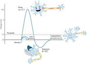
Fig. 1. Illustration for quantum-like representation of uncertainty generated by neuron’s action potential (originally published in Khrennikov et al. (2018)).
Hacemos hincapié en que el modelado de tipo cuántico eleva el papel de la conveniencia y la simplicidad de la representación cuántica de estados y observables. (Ignoramos pragmáticamente el problema de la interrelación de CP y QP). En particular, el espacio de estado cuántico tiene una estructura lineal y los modelos lineales son más simples. La transición de la dinámica no lineal clásica de los procesos electroquímicos en biosistemas a la dinámica lineal cuántica esencialmente acelera la evolución del estado (Sección 8.4). Sin embargo, en este marco, "estado" es el estado de información cuántica de un biosistema utilizado para el procesamiento de la incertidumbre cuántica especial (Sección 8.2).
Observaciones
En los libros de texto sobre mecánica cuántica, se suele señalar que la principal característica distintiva de la teoría cuántica es la presencia de observables incompatibles. Recordemos que dos observables 
 y son incompatibles si es imposible asignarles valores conjuntamente. En el modelo probabilístico, esto lleva a la imposibilidad de determinar su distribución de probabilidad conjunta (JPD). Los ejemplos básicos de observables incompatibles son la posición y el momento de un sistema cuántico, o las proyecciones de espín (o polarización) en diferentes ejes. En el formalismo matemático, la incompatibilidad se describe como la no conmutatividad de los operadores hermitianos.
  y
y  representando observables, i.e.,
 ![{\displaystyle [{\hat {A}},{\hat {B}}]\neq 0}](https://wikimedia.org/api/rest_v1/media/math/render/svg/9ca6253a4b7d1fed6f0b83ee4f14d05f740af438)
Aquí nos referimos al modelo original y aún básico y ampliamente utilizado de observables cuánticos, Von Neumann 1955[24] (Sección 3.2).
La incompatibilidad-no conmutatividad se usa ampliamente en la física cuántica y los observables físicos básicos, como las proyecciones de posición y momento, espín y polarización, se representan tradicionalmente en este paradigma, mediante operadores hermitianos. También señalamos numerosas aplicaciones de este enfoque a la cognición, la psicología, la toma de decisiones (Khrennikov, 2004a[25], Busemeyer y Bruza, 2012[26], Bagarello, 2019[27]) (ver especialmente el artículo (Bagarello et al., 2018[28]) dedicado a la cuantificación de la Relaciones de incertidumbre de Heisenberg en la toma de decisiones). Aún así, puede que no sea lo suficientemente general para nuestro propósito: para el modelado de tipo cuántico en biología, ningún tipo de bioestadística no clásica se puede delegar fácilmente al modelo de observaciones de von Neumann. Por ejemplo, ni siquiera los efectos cognitivos más básicos pueden describirse de manera coherente con el modelo de observación estándar (Khrennikov et al., 2014[29], Basieva y Khrennikov, 2015[30]).
Exploraremos teorías más generales de las observaciones basadas en instrumentos cuánticos (Davies y Lewis, 1970[17], Davies, 1976[18], Ozawa, 1984[19], Yuen, 1987[20], Ozawa, 1997[21], Ozawa, 2004[31], Okamura y Ozawa, 2016[23]) y encontraremos herramientas útiles para aplicaciones al modelado de efectos cognitivos (Ozawa y Khrennikov, 2020a[32], Ozawa y Khrennikov, 2020b[33]). Discutiremos esta pregunta en la Sección 3 y la ilustraremos con ejemplos de cognición y biología molecular en las Secciones 6, 7. En el marco de la teoría cuántica de instrumentos, el punto crucial no es la conmutatividad frente a la no conmutatividad de los operadores que representan simbólicamente observables, sino la forma matemática de la transformación de estado resultante de la acción posterior de la (auto)observación. En el enfoque estándar, esta transformación viene dada por una proyección ortogonal en el subespacio de vectores propios correspondientes a la salida de la observación. Este es el postulado de proyección. En la teoría cuántica de instrumentos, las transformaciones de estado son más generales.
El cálculo de instrumentos cuánticos está estrechamente relacionado con la teoría de los sistemas cuánticos abiertos (Ingarden et al., 1997[34]), sistemas cuánticos que interactúan con los entornos. Hacemos notar que en algunas situaciones, los sistemas físicos cuánticos pueden requerir (al menos aproximadamente) aislados. Sin embargo, los biosistemas son muy abiertos. Como destaca Schrödinger (1944[35]), un biosistema completamente aislado está muerto. Esto último explica por qué la teoría de los sistemas cuánticos abiertos y, en particular, el cálculo de instrumentos cuánticos juegan el papel básico en las aplicaciones a la biología, como el aparato matemático de la biología cuántica de la información (Asano et al., 2015a[36]).
Dentro de la teoría de los sistemas cuánticos abiertos, modelamos la evolución epigenética (Asano et al., 2012b[37], Asano et al., 2015b[38]) (Secciones 9, 11.2) y el desempeño de las funciones psicológicas (cognitivas) realizadas por el cerebro (Asano et al., 2015b). 2011[39], Asano et al., 2015b[38], Khrennikov et al., 2018[40]
Para biólogos matemáticamente suficientemente bien educados, pero sin conocimiento en física, podemos recomendar un libro (Khrennikov, 2016a[41]) que combina las presentaciones de CP y QP con una breve introducción al formalismo cuántico, incluida la teoría de los instrumentos cuánticos y las probabilidades condicionales.
2. Probabilidad clásica versus cuántica
CP fue formalizada matemáticamente por Kolmogorov (1933)[15] Este es el cálculo de medidas de probabilidad, donde un peso no negativo se asigna a cualquier evento . La principal propiedad de CP es su aditividad: si dos eventos
  son disjuntos, entonces la probabilidad de disyunción de estos eventos es igual a la suma de probabilidades:
|
|

|
|
QP es el cálculo de amplitudes complejas o, en el formalismo abstracto, vectores complejos. Así, en lugar de operaciones sobre medidas de probabilidad, se opera con vectores. Podemos decir que QP es un modelo vectorial de razonamiento probabilístico. Cada amplitud compleja  da la probabilidad por la regla de Born: La probabilidad se obtiene como el cuadrado del valor absoluto de la amplitud compleja.
|
|

|
|
(para la formalización del espacio de Hilbert, consulte la Sección 3.2, fórmula (7)). Al operar con amplitudes de probabilidad complejas, en lugar de la operación directa con probabilidades, se pueden violar las leyes básicas de CP.
En CP, la fórmula de probabilidad total (FTP) se obtiene usando la aditividad de la probabilidad y la fórmula de Bayes, la definición de probabilidad condicional,  ,
, 
Considere el par, y , de variables aleatorias clásicas discretas. Entonces
|
|

|
|
Así, en CP la -La distribución de probabilidad se puede calcular a partir de la -probabilidad y las probabilidades condicionales

En QP, el FTP clásico es perturbado por el término de interferencia (Khrennikov, 2010[42]); para observables cuánticos dicotómicos y Del tipo von Neumann, es decir, dado por operadores hermitianos y , la versión cuántica de FTP tiene la forma:
|
|

|

|
|
|

|

|
Si el término de interferencia7 es positivo, entonces el cálculo QP generaría una probabilidad mayor que su contraparte CP dada por el FTP clásico (2). En particular, esta amplificación de probabilidad es la base de la supremacía de la computación cuántica.
Hay una gran cantidad de datos estadísticos de la psicología cognitiva, la toma de decisiones, la biología molecular, la genética y la epigenética que demuestran que los biosistemas, desde las proteínas y las células (Asano et al., 2015b[38]) hasta los humanos (Khrennikov, 2010[43], Busemeyer y Bruza, 2012[26]) utilizan esta amplificación y operar con actualizaciones que no sean de CP. Continuamos nuestra presentación con tales ejemplos.
3. Instrumentos cuánticos
3.1. Algunas palabras sobre el formalismo cuántico
Denotamos por  un espacio complejo de Hilbert. Por simplicidad, asumimos que es de dimensión finita. Estados puros de un sistema
  están dados por vectores normalizados de y estados mixtos por operadores de densidad (operadores semidefinidos positivos con traza unitaria). El espacio de los operadores de densidad se denota por (). El espacio de todos los operadores lineales en se denota con el símbolo
  . A su vez, este es un espacio lineal. Además, es el espacio complejo de Hilbert con el producto escalar,
 . Consideramos operadores lineales actuando en . Se llaman superoperadores.
La dinámica del estado puro de un sistema cuántico aislado se describe mediante la ecuación de Schrödinger:
|
|

|

|
dónde  es el hamiltoniano del sistema. Esta ecuación implica que el estado puro
  evoluciona unitariamente
  , donde
  Es un grupo paramétrico de operadores unitarios. ,
 . En física cuántica, hamiltoniano está asociado con la energía observable. La misma interpretación se utiliza en biofísica cuántica (Arndt et al., 2009).[44] Sin embargo, en nuestro modelo cuántico que describe el procesamiento de información en biosistemas, el operador no tiene acoplamiento directo con la energía física. Este es el generador de evolución que describe las interacciones de información.
La dinámica de Schrödinger para un estado puro implica que la dinámica de un estado mixto (representado por un operador de densidad) se describe mediante la ecuación de von Neumann:
|
|
![{\displaystyle {\frac {d{\hat {\rho }}}{dt}}(t)=-i[{\hat {\mathcal {H}}},{\hat {\rho }}(t)],{\hat {\rho }}(0)={\hat {\rho }}_{0}}](https://wikimedia.org/api/rest_v1/media/math/render/svg/46cb03104a69d14e36fd6776550cc38a492b9634)
|

|
3.2. Formalismo de Von Neumann para observables cuánticos
En el formalismo cuántico original (Von Neumann, 1955),[45] físico observable está representado por un operador hermitiano .Consideramos solo operadores con espectros discretos : dónde
dónde  es el proyector sobre el subespacio de correspondiente al valor propio
  . Supongamos que el estado del sistema se representa matemáticamente mediante un operador de densidad
  . Entonces la probabilidad de obtener la respuestar viene dada por la regla de Born
|
|
![{\textstyle Pr\{A=x||\rho \}=Tr[{\widehat {E}}^{A}(x)\rho ]=Tr[{\widehat {E}}^{A}(x)\rho {\widehat {E}}^{A}(x)]}](https://wikimedia.org/api/rest_v1/media/math/render/svg/dffc6a2b1bbc16202b1abab10b045f1fcc304c04)
|

|
y de acuerdo con el postulado de proyección, el estado posterior a la medición se obtiene a través de la transformación de estado:
|
|

|

|
Para comodidad del lector, presentamos estas fórmulas para un estado inicial puro  . La regla de Born tiene la forma:
|
|

|

|
La transformación de estado viene dada por el postulado de proyección:
|
|

|

|
Aquí el operador observable (su descomposición espectral) determina de forma única las transformaciones del estado de retroalimentación para resultados
|
|

|

|
El mapa  dada por (9) es el ejemplo más simple (pero muy importante) de instrumento cuántico.
3.3. Actualización de estado no proyectivo: instrumentos atómicos
En general, las propiedades estadísticas de cualquier medida se caracterizan por
- la distribución de probabilidad de salida
 , la distribución de probabilidad de la salida de la medida en el estado de entrada ;
- la reducción del estado cuántico
 ,el cambio de estado desde el estado de entrada al estado de salida condicionado al resultado
  de la medida
En la formulación de von Neumann, las propiedades estadísticas de cualquier medida de un observable están determinadas únicamente por la regla de Born (5) y el postulado de proyección (6), y están representadas por el mapa (9), un instrumento de tipo von Neumann. Sin embargo, la formulación de von Neumann no refleja el hecho de que el mismo representado por el operador hermitiano en puede medirse de muchas maneras.8 Formalmente, tales esquemas de medición están representados por instrumentos cuánticos.
Ahora, consideramos los instrumentos cuánticos más simples del tipo no von Neumann, conocidos como instrumentos atómicos. Comenzamos recordando la noción de POVM (medida valorada por el operador de probabilidad); restringimos las consideraciones a POVM con un dominio de definición discreto  . POVMes un mapa
  tal que para cada
  ,
, es un operador hermitiano contractivo positivo (llamado efecto) (es decir,,
 o cualquier ), y la condición de normalización

sostiene, donde  es el operador de la unidad. Se supone que para cualquier medida, la distribución de probabilidad de salida
  es dado por
|
|
![{\textstyle Pr\{{\text{x}}=x||\rho \}=Tr[{\hat {D}}(x)\rho ]}](https://wikimedia.org/api/rest_v1/media/math/render/svg/229874a62a1d92651c5a1e60265399c0e969dd05)
|

|
dónde  es un POVM. Para instrumentos atómicos, se supone que los efectos se representan concretamente en la forma
|
|

|

|
dónde  Es un operador lineal en ( .Por lo tanto, la condición de normalización tiene la forma
  .9 La regla de Born se puede escribir de manera similar a (5):
|
|
![{\textstyle Pr\{{\text{x}}=x||\rho \}=Tr[{V}(x)\rho {V}^{*}(x)]}](https://wikimedia.org/api/rest_v1/media/math/render/svg/cd51eeb8f4e5b9cd30d856040525bb2be6f94c0b)
|

|
Se supone que la transformación del estado posterior a la medición se basa en el mapa:
| *
|

|

|
por lo que la reducción del estado cuántico viene dada por
| *
|
![{\textstyle \rho \rightarrow \rho _{({\text{x}}=x)}={\frac {{\mathcal {L}}_{A}(x)\rho }{Tr[{\mathcal {L}}_{A}(x)\rho ]}}}](https://wikimedia.org/api/rest_v1/media/math/render/svg/6c622ed9f3472b9bc13374d7bd37e7da807ab612)
|

|
El mapa  dada por (13) es un instrumento cuántico atómico. Observamos que la regla de Born (12) se puede escribir en la forma
| *
|
![{\textstyle Pr\{{\text{x}}=x||\rho \}=Tr[\Im _{A}(x)\rho ]}](https://wikimedia.org/api/rest_v1/media/math/render/svg/586d4e469a1b620c551892a44aab492958653f02)
|
 f f
|
Dejar ser un operador hermitiano en . Considere un POVM  con el dominio de definición dado por el espectro de . Este POVM representa una medida de observable si se cumple la regla de Born:
|
|
![{\textstyle Pr\{{\text{A}}=x||\rho \}=Tr[{\widehat {D}}^{A}(x)\rho ]=Tr[{\widehat {E}}^{A}(x)\rho ]}](https://wikimedia.org/api/rest_v1/media/math/render/svg/b9a8550566f3459e7cddbf180fcde8f50d4c299b)
|

|
Por lo tanto, en principio, las probabilidades de los resultados todavía están codificadas en la descomposición espectral del operador O en otras palabras operadores  deben seleccionarse de tal manera que generen las probabilidades correspondientes a la descomposición espectral de la representación simbólica de observables ,es decir., está determinada únicamente por como
  . Podemos decir que este operador solo lleva información sobre las probabilidades de los resultados, en contraste con el esquema de von Neumann, el operador no codifica la regla de actualización de estado. Para un instrumento atómico, las mediciones del observable tiene la distribución de probabilidad de salida única según la regla de Born (16), pero tiene muchas reducciones de estado cuántico diferentes dependiendo de la descomposición del efecto
  de una manera que
|
|
![{\textstyle \rho \rightarrow \rho _{({\text{A}}=x)}={\frac {{V}(x)\rho V(x)^{*}}{Tr[{V}(x)\rho V(x)^{*}]}}}](https://wikimedia.org/api/rest_v1/media/math/render/svg/ba54c1d316d7ab6acff66de4f7dc854ac7eda6f0)
|

|
3.4. Teoría general (Davies-Lewis-Ozawa)
Finalmente, formulamos la noción general de instrumento cuántico. Un superoperador actuando en se llama positivo si mapea el conjunto de operadores semidefinidos positivos en sí mismo. Resaltamos que, para cada  dado por (13) puede considerarse como un mapa lineal positivo.
Generalmente cualquier mapa  , donde para cada
  , el mapa
  es un superoperador positivo se llama Davies-Lewis (Davies y Lewis, 1970)[46] instrumento cuántico.
Aquí índice  denota el observable acoplado a este instrumento. Las probabilidades de -los resultados vienen dados por la regla de Born en forma (15) y la actualización de estado por transformación (14). Sin embargo, Yuen (1987[47]) señaló que la clase de instrumentos de Davies-Lewis es demasiado general para excluir instrumentos físicamente irrealizables. Ozawa (1984[48]) introdujo la importante condición adicional para asegurar que cada instrumento cuántico sea físicamente realizable. Esta es la condición de la positividad completa.
Un superoperador se llama completamente positivo si su extensión natural  al producto tensorial
  es de nuevo un superoperador positivo en
  . Un mapa , donde para cada ,el mapa es un superoperador completamente positivo se llama Davies-Lewis-Ozawa (Davies y Lewis 1970,[49] Ozawa, 1984[48]instrumento cuántico o simplemente instrumento cuántico. Como veremos en la Sección 4, la positividad completa es condición suficiente para que un instrumento sea físicamente realizable. Por otro lado, la necesidad se deriva de la siguiente manera (Ozawa, 2004)[50]
cada observable de un sistema  se identifica con el observable
  de un sistema
  con cualquier sistema
  Externo a .10
Entonces, cada instrumento físicamente realizable  medición debe identificarse con el instrumento
  medición
  tal que
 . Esto implica que
  es de nuevo un superoperador positivo, por lo que Es completamente positivo.
Del mismo modo, cualquier instrumento físicamente realizable sistema de medición debe tener su instrumento extendido sistema de medición para cualquier sistema externo .Esto se cumple sólo si es completamente positivo. Así, la positividad completa es una condición necesaria para para describir un instrumento físicamente realizable.
4. Instrumentos cuánticos del esquema de medidas indirectas.
El modelo básico para la construcción de instrumentos cuánticos se basa en el esquema de medidas indirectas. Este esquema formaliza la siguiente situación: los resultados de la medición se generan a través de la interacción de un sistema con un aparato de medida  .Este aparato consiste en un dispositivo físico complejo que interactúa con y un puntero que muestra el resultado de la medición, digamos girar hacia arriba o hacia abajo. Un observador solo puede ver las salidas del puntero y asocia estas salidas con los valores del observable. para el sistema .Así, el esquema de medición indirecta implica:
- los estados del sistemas y el aparato
- El operador
 representando la dinámica de interacción para el sistema
- el metro observable
 dando salidas del puntero del aparato .
Un modelo de medición indirecta, introducido en Ozawa (1984)[48] como un "proceso de medición (general)", es un cuádruple

que consta de un espacio de Hilbert  ,un operador de densidad
  , Un operador unitario sobre el producto tensorial de los espacios de estado de y
  y un operador hermitiano on . Por este modelo de medida, el espacio de Hilbert describe los estados del aparato , El operador unitario describe la evolución temporal del sistema compuesto , El operador de densidad
  describe el estado inicial del aparato , y el operador hermitiano describe el metro observable del aparato . Entonces, la distribución de probabilidad de salida.
  en el estado del sistema es dado por
|
|
![{\displaystyle Pr\{A=x\|\rho \}=Tr[{\Bigl (}I\otimes E^{M}{^{_{A}}(x){\Bigr )}}U(\rho \otimes \sigma )U^{*}]}](https://wikimedia.org/api/rest_v1/media/math/render/svg/4f3cd4375be3c41ac3dd1be33638372ab6f99ec1)
|

|
dónde  es la proyección espectral de para el valor propio .
El cambio de estado del sistema causado por la medición para el resultado  se representa con la ayuda del mapa en el espacio de operadores de densidad definidos como
|
|
![{\displaystyle {\mathcal {P}}_{A}(x)\rho =Tr_{\mathcal {H}}[{\Bigl (}I\otimes E^{M}{^{_{A}}(x){\Bigr )}}U(\rho \otimes \sigma )U^{*}]}](https://wikimedia.org/api/rest_v1/media/math/render/svg/30510a056cd9495c058447715652efe281343aee)
|

|
dónde  es la traza parcial sobre . Entonces, el mapa resultar ser un instrumento cuántico. Así, las propiedades estadísticas de la medida realizada por cualquier modelo de medida indirecta se describe mediante una medida cuántica. Resaltamos que, a la inversa, cualquier instrumento cuántico puede representarse mediante el modelo de medición indirecta (Ozawa, 1984).[48]Así, los instrumentos cuánticos caracterizan matemáticamente las propiedades estadísticas de todas las medidas cuánticas físicamente realizables.
5. Modelado del proceso de sensación-percepción dentro del esquema de medición indirecta
H. von Helmholtz estableció los fundamentos de la teoría de la inferencia inconsciente para la formación de impresiones visuales en el siglo XIX. Aunque von Helmholtz estudió principalmente la sensación-percepción visual, también aplicó su teoría a otros sentidos hasta culminar en la teoría de la inferencia del inconsciente social. Por von Helmholtz aquí hay dos etapas del proceso cognitivo, y discriminan entre sensación y percepción de la siguiente manera:
- La sensación es una señal que el cerebro interpreta como un sonido o una imagen visual, etc.
- La percepción es algo que debe interpretarse como una preferencia o atención selectiva, etc.
En el esquema de medición indirecta, las sensaciones representan los estados del sistema de sensaciones del ser humano y el sistema de percepción desempeña el papel del aparato de medición. El operador unitario describe el proceso de interacción entre los estados de sensación y percepción. Este modelado cuántico del proceso de sensación-percepción se presentó en papel (Khrennikov, 2015)[51]con aplicación a la percepción biestable y datos experimentales del artículo (Asano et al., 2014).[52]
6. Modelado de efectos cognitivos
En las ciencias cognitivas y sociales, el siguiente grupo de opiniones se conoce como el ejemplo básico del efecto de orden. Este es el grupo de opinión Clinton-Gore (Moore, 2002).[53] En este experimento, a los ciudadanos estadounidenses se les hizo una pregunta a la vez, por ejemplo,
 "¿Es Bill Clinton honesto y confiable?"
 "¿Es Al Gore honesto y confiable?"
Se calcularon dos distribuciones de probabilidad secuenciales sobre la base de los datos estadísticos experimentales,  y
y  (primera pregunta y luego pregunta y viceversa).
6.1. Efecto de orden para interrogatorio secuencial
Los datos estadísticos de este experimento demostraron el efecto QOE del orden de las preguntas, la dependencia de la distribución de probabilidad conjunta secuencial para las respuestas a las preguntas en su orden.  . Observamos que en el modelo CP estas distribuciones de probabilidad coinciden:

dónde  es un espacio muestral
  y es una medida de probabilidad.
QOE estimula la aplicación del cálculo QP a la cognición, ver artículo (Wang y Busemeyer, 2013).[54]Los autores de este artículo enfatizaron que la característica no conmutativa de las probabilidades conjuntas se puede modelar mediante el uso de la no conmutatividad de observables cuánticos incompatibles.  representado por operadores hermitianos
  . Observable representa la pregunta de Clinton y observable representa la pregunta de Gore. En este modelo, QOE es idéntica incompatibilidad-no conmutatividad de observables:
![{\displaystyle [{\widehat {A}},{\widehat {B}}]\neq 0}](https://wikimedia.org/api/rest_v1/media/math/render/svg/1e9db6c1b5e87d54bf434dd1a9c5e27aec96f01b)
6.2. Efecto de replicabilidad de respuestas para preguntas secuenciales
El enfoque basado en la identificación del efecto de orden con representación no conmutativa de preguntas(Wang and Busemeyer, 2013)[55] fue criticado en papel (Khrennikov et al., 2014).[56] Para discutir este artículo, recordamos la noción de replicabilidad de la respuesta. Supongamos que a una persona, digamos John, se le hace una pregunta y supongamos que él responde, por ejemplo, "sí". Si inmediatamente después de esto, se le vuelve a hacer la misma pregunta, entonces responde "sí" con probabilidad uno. A esta propiedad la llamamos  replicabilidad de la respuesta. En la física cuántica, la replicabilidad de la respuesta se expresa mediante el postulado de proyección. La encuesta de opinión de Clinton-Gore, así como los experimentos típicos de toma de decisiones, satisfacen replicabilidad de la respuesta. La toma de decisiones también tiene otra característica: replicabilidad de la respuesta. Supongamos que después de responder a la -pregunta con la respuesta "sí", a John se le hace otra pregunta . Él respondió con alguna respuesta. Y luego se le pregunta de nuevo. En el grupo de opinión social antes mencionado, John repite su respuesta original a ,“sí” (con probabilidad uno).
Este fenómeno de comportamiento que llamamos  replicabilidad de la respuesta. Combinación de con y
  la replicabilidad de la respuesta se denomina efecto de replicabilidad de la respuesta RRE.
6.3.“QOE+RRE”: descrito por instrumentos cuánticos de tipo no proyectivo
En papel (Khrennikov et al., 2014),[56] se demostró que usando el cálculo de von Neumann es imposible combinar RRE con QOE. Para generar QOE, operadores hermitianos Debe ser no conmutativo, pero este último destruye replicabilidad de la respuesta de . Este fue un resultado bastante inesperado. Incluso dio la impresión de que, aunque los efectos cognitivos básicos pueden modelarse cuánticamente por separado, sus combinaciones no pueden describirse mediante el formalismo cuántico.
Sin embargo, recientemente se demostró que la teoría de los instrumentos cuánticos proporciona una solución simple de la combinación de los efectos QOE y RRE, ver Ozawa y Khrennikov (2020a)[57] para la construcción de dichos instrumentos. Estos instrumentos son de tipo no proyectivo. Así, la esencia de QOE no está en la estructura de los observables, sino en la estructura de la transformación de estado generada por la retroalimentación de las medidas. QOE no se trata de la medición conjunta y la incompatibilidad (no conmutatividad) de los observables, sino de la medición secuencial de los observables y la actualización secuencial del estado (mental). Instrumentos cuánticos que se utilizan en Ozawa y Khrennikov (2020a)[57] para combinar QOE y RRE corresponden a la medición de observables representados por operadores de conmutación .Además, es posible demostrar que (bajo restricción matemática natural) QOE y RRE pueden modelarse conjuntamente solo con la ayuda de instrumentos cuánticos para conmutar observables.
6.4. Realismo mental
Desde el comienzo de la mecánica cuántica, la no conmutatividad de los operadores. representando observables fue considerada como la representación matemática de su incompatibilidad. En términos filosóficos, esta situación se trata como imposibilidad de la descripción realista. En la ciencia cognitiva, esto significa que existen estados mentales tales que un individuo no puede asignar los valores definidos a ambos observables (por ejemplo, preguntas). La descripción matemática de QOE con observables representados por operadores no conmutativos (en el esquema de von Neumann) en Wang y Busemeyer(2013)[58] y Wang et al. (2014)[59] dio la impresión de que este efecto implica el rechazo del realismo mental. El resultado deOzawa y Khrennikov (2020a)[60] demuestra que, a pesar de QOE experimentalmente bien documentado, el realismo mental no necesita ser rechazado. QOE se puede modelar dentro de la imagen realista dada matemáticamente por la distribución de probabilidad conjunta de observables y ,pero con la acción no conmutativa de los instrumentos cuánticos actualizando el estado mental:
|
|
![{\displaystyle [{\mathcal {J_{A}(x)}},{\mathcal {J_{B}(x)}}]={\mathcal {J_{A}(x)}}{\mathcal {J_{B}(x)}}-{\mathcal {J_{B}(x)}},{\mathcal {J_{A}(x)}}\neq 0}](https://wikimedia.org/api/rest_v1/media/math/render/svg/361fd78b0a02b9327edd624db3524e24db18c76b)
|

|
Este es un buen lugar para comentar que si, para algún estado ![{\displaystyle \rho ,[\Im _{A}(x),\Im _{B}(x)]\rho =0}](https://wikimedia.org/api/rest_v1/media/math/render/svg/8e92482fee8da2743e673c367d456a5072ea1ade) , entonces QOE desaparece, incluso si
, entonces QOE desaparece, incluso si ![{\displaystyle [\Im _{A}(x),\Im _{B}(x)]\neq 0}](https://wikimedia.org/api/rest_v1/media/math/render/svg/f79e1311a59bf9e0fb79419b798b7ed5b018f921) .Esto puede considerarse como la formulación correcta de la declaración de Wang-Bussemeyer sobre la conexión de QOE con la no conmutatividad. En lugar de la no conmutatividad de los operadores
.Esto puede considerarse como la formulación correcta de la declaración de Wang-Bussemeyer sobre la conexión de QOE con la no conmutatividad. En lugar de la no conmutatividad de los operadores  y
y  representando simbólicamente observables cuánticos, uno tiene que hablar de no conmutatividad de los instrumentos cuánticos correspondientes.
7. Genética: interferencia en el metabolismo de glucosa/lactosa
En papel (Asano et al., 2012a),[56]se desarrolló un modelo de tipo cuántico que describe la regulación génica del metabolismo de la glucosa/lactosa en la bacteria Escherichia coli.11 Hay varios tipos de E. coli caracterizados por el sistema metabólico. Se demostró que el tipo concreto de E. coli puede ser descrito por los operadores lineales bien determinados; encontramos las cantidades de operadores invariantes que caracterizan cada tipo. Tales cantidades de operadores invariantes se pueden calcular a partir de los datos estadísticos obtenidos. Entonces, la representación de tipo cuántico se reconstruyó a partir de datos experimentales.
Consideremos un sistema de eventos  significa el evento en que E. coli activa su operón de lactosa, es decir, el evento en que se produce -galactosidasa a través de la transcripción del ARNm de un gen en el operón de lactosa;
  significa el evento de que E. coli no active su operón de lactosa.
Este sistema de eventos corresponde a una activación observable que es matemáticamente representada por un instrumento cuántico  . Considere ahora otro sistema de eventos
  dónde
dónde  significa el evento de que una bacteria E. coli detecta una molécula de lactosa en el entorno circundante de la célula, significa
  detección de una molécula de glucosa. Este sistema de eventos corresponde a la detección observable
  que está representado por un instrumento cuántico
 .
.
En este modelo, la interacción-reacción de la bacteria con el entorno de glucosa/lactosa se describe como una acción secuencial de dos instrumentos cuánticos, primero la detección y luego la activación. Como se mostró en Asano et al.(2012a)[56], para cada tipo concreto de bacteria E. coli, estos instrumentos cuánticos pueden reconstruirse a partir de los datos experimentales; Asano et al. (2012a),[56]la reconstrucción se realizó para el tipo W3110 de la bacteria E. coli. El FTP clásico con observables  and
and  se viola, el término de interferencia, ver (2), se calculó (Asano et al., 2012a).[56]
8. Sistemas cuánticos abiertos: interacción de un biosistema con su entorno
Como ya se enfatizó, cualquier biosistema es fundamentalmente abierto. Por lo tanto, la dinámica de su estado debe modelarse a través de una interacción con el entorno circundante.  . los estados de y están representados en los espacios de Hilbert y . el sistema compuesto
  se representa en el producto tensorial espacios de Hilbert. Este sistema se trata como un sistema aislado y, de acuerdo con la teoría cuántica, la dinámica de su estado puro se puede describir mediante la ecuación de Schrödinger:
|
|

|

|
dónde es el estado puro del sistema y  es su hamiltoniano. Esta ecuación implica que el estado puro evoluciona unitariamente: . Aquí . hamiltoniano (generador de evolución) que describe las interacciones de información tiene la forma
  , dónde
  ,
, son hamiltonianos de los sistemas y
  es la interacción hamiltoniana.12 Esta ecuación implica que la evolución del operador de densidad
  del sistema se describe mediante la ecuación de von Neumann:
|
|
![{\displaystyle {\tfrac {d{\widehat {R}}}{dt}}(t)=-i[{\widehat {H}},{\widehat {R}},(t)],{\widehat {R}}(0)={\widehat {R}}_{0}}](https://wikimedia.org/api/rest_v1/media/math/render/svg/f5360ff03d80449ad8d6c2745e7b1ce43093e52c)
|

|
Sin embargo, el estado es demasiado complejo para cualquier análisis matemático: el entorno incluye demasiados grados de libertad. Por lo tanto, sólo nos interesa el estado de ; su dinámica se obtiene mediante el seguimiento del estado de w.r.t. los grados de libertad de :
|
|

|

|
Generalmente esta ecuación, la ecuación maestra cuántica, es matemáticamente muy complicada. En las aplicaciones se utiliza una variedad de aproximaciones.
8.1. Modelo cuántico de Markov: ecuación de Gorini-Kossakowski-Sudarshan-Lindblade
La aproximación más simple de la ecuación maestra cuántica (23) es la dinámica cuántica de Markov dada por la ecuación de Gorini-Kossakowski-Sudarshan-Lindblad (GKSL) (Ingarden et al., 1997)[61] (en física, comúnmente se le llama simplemente la ecuación de Lindblad; esta es la ecuación maestra cuántica más simple):
|
|
![{\displaystyle {\tfrac {d{\widehat {\rho }}}{dt}}(t)=-i[{\widehat {H}},{\widehat {\rho }},(t)]+{\widehat {L}}[{\widehat {\rho }}(t),{\widehat {\rho }}(0)={\widehat {\rho }}_{0}}](https://wikimedia.org/api/rest_v1/media/math/render/svg/8ced507a031874df17864ed03824140ff695bf48)
|

|
donde operador hermitiano (hamiltoniano)  Describe la dinámica interna de y el superoperador
  , actuando en el espacio de los operadores de densidad, describe una interacción con el entorno . Este superoperador a menudo se llama Lindbladian. La ecuación GKSL es una ecuación maestra cuántica para la dinámica markoviana. En este artículo, no tenemos posibilidad de explicar la noción de markovianidad cuántica con más detalle. La ecuación maestra cuántica (23) describe, en general, dinámicas no markovianas.
8.2. Funciones biológicas en el marco cuántico de Markov
Pasamos a la dinámica de sistemas abiertos con la ecuación GKSL. En nuestro modelo, hamiltoniano y Lindbladian representan alguna función biológica especial  (ver Khrennikov et al., 2018)[62]para detalles. Su funcionamiento resulta de la interacción de flujos de información internos y externos. En las Secciones 10, 11.3, es alguna función psicológica; en el caso más simple representa una pregunta hecha a (digamos que es un ser humano). En la Sección 7, es la regulación génica del metabolismo de la glucosa/lactosa en la bacteria Escherichia coli. En las Secciones 9, 11.2, representa el proceso de mutación epigenética. Función simbólicamente biológica se representa como un observable cuántico: operador hermitiano
  con la descomposición espectral
  ,dónde etiqueta las salidas de .La teoría de la dinámica de estado cuántica de Markov describe el proceso de generación de estos resultados.
En el modelo matemático (Asano et al., 2015b[63], Asano et al., 2017b[64], Asano et al., 2017a[65], Asano et al., 2015a[66], Asano et al., 2012b[67], Asano et al., 2011[68], Asano et al. ., 2012a[69]), los resultados de la función biológica se generan acercándose a un estado estable de la dinámica GKSL:
|
|

|

|
tal que coincide con la descomposición espectral de ,es decir.,
|
|

|

|
dónde
|
|

|
|
Esto significa que  es diagonal en una base ortonormal que consta de vectores propios de . Este estado, o más precisamente, esta descomposición del operador de densidad ,es la mezcla estadística clásica de los estados básicos de información que determinan esta función biológica. Las probabilidades en la descomposición de estados (26) se interpretan estadísticamente.
Considere un gran conjunto de biosistemas con el estado  interactuando con el medio ambiente . (Recordemos que matemáticamente la interacción está codificada en el Lindbladian ) Como resultado de esta interacción, la función biológica produce salida con probabilidad
  .Observamos que en los términos del operador la probabilidad se expresa como
Esta interpretación se puede aplicar incluso a un solo biosistema que se encuentra con el mismo entorno muchas veces.
Cabe señalar que el estado límite expresa la estabilidad con respecto a la influencia del entorno concreto .Por supuesto, en el mundo real nunca se alcanzaría el estado límite. La fórmula matemática (25) describe el proceso de estabilización, amortiguación de fluctuaciones. Pero, nunca desaparecerían por completo con el tiempo.
Observamos que un estado estacionario satisface la ecuación GKSL estacionaria:
|
|
![{\displaystyle i[{\widehat {H}},{\widehat {\rho }}_{steady}]={\widehat {L}}[{\widehat {\rho }}_{steady}]}](https://wikimedia.org/api/rest_v1/media/math/render/svg/9f2a348496cb945fd0a1351418b60d74ad83430c)
|

|
También es importante señalar que, en general, un estado estacionario de la ecuación maestra cuántica no es único, depende de la clase de condiciones iniciales.
8.3.Funcionamiento de las funciones biológicas a través de la decoherencia
Para concretar las consideraciones anteriores, consideremos un estado cuántico puro como estado inicial. Supongamos que una función biológica es dicotómica,  , y está representado simbólicamente por el operador hermitiano que es diagonal en base ortonormal
  ,
, .(Consideramos el espacio de estado bidimensional, el espacio qubit). Deje que el estado inicial tenga la forma de superposición
|
|

|

|
dónde  . La dinámica del maestro cuántico no es una dinámica de estado puro: tarde o temprano (de hecho, muy pronto), esta superposición que representa un estado puro se transferirá a una matriz de densidad que representa un estado mixto. Por lo tanto, desde el principio es útil representar la superposición (28) en términos de una matriz de densidad:
|
|

|

|
La pureza del estado, la superposición, se caracteriza por la presencia de términos distintos de cero fuera de la diagonal.
La superposición codifica la incertidumbre con respecto a la base del estado concreto, en nuestro caso ,.Inicialmente función biológica estaba en el estado de incertidumbre entre dos opciones  . Esta es una incertidumbre cuántica (como) genuina. Incertidumbre, sobre posibles acciones en el futuro. Por ejemplo, para la función psicológica (Sección 10) representando responder a alguna pregunta, digamos "comprar una propiedad"(
  ) y su negacion (
  ) , una persona cuyo estado se describe por superposición (28) no está seguro de actuar con ( ) o con ( ) . Así, un estado de tipo superposición describe la incertidumbre individual, es decir, la incertidumbre asociada con el biosistema individual y no con un conjunto de biosistemas; con el solo acto de funcionamiento de y no con una gran serie de tales actos.
Resolución de la incertidumbre con respecto a  se caracteriza por lavar los términos fuera de la diagonal en (29) La dinámica cuántica (24) suprime los términos fuera de la diagonal y, finalmente, se genera una matriz de densidad diagonal que representa un estado estacionario de estos sistemas dinámicos:
|
|

|

|
Esta es una mezcla estadística clásica. Describe un conjunto de biosistemas; estadísticamente generan salidas  con probabilidades
  .De la misma manera, la interpretación estadística se puede utilizar para un solo sistema que realiza -funcionando en diferentes instancias de tiempo (para una larga serie de tiempo).
En física cuántica, el proceso de eliminar los elementos fuera de la diagonal en una matriz de densidad se conoce como proceso de decoherencia. Así, el modelo descrito de puede llamarse funcionamiento de la función biológica a través de la decoherencia.
8.4.Linealidad de la representación cuántica: aceleración exponencial del funcionamiento biológico
El modelado de tipo cuántico no afirma que los biosistemas sean fundamentalmente cuánticos. Una imagen más natural es que son sistemas biofísicos clásicos complejos y el modelo cuántico proporciona la representación de información de procesos biofísicos clásicos, en genes, proteínas, células, cerebros. Una de las ventajas de esta representación es su linealidad. El espacio de estado cuántico es un espacio de Hilbert complejo y las ecuaciones dinámicas son ecuaciones diferenciales lineales. Para espacios de estado de dimensión finita, estas son solo ecuaciones diferenciales ordinarias con coeficientes complejos (por lo tanto, el lector no debe temer nombres tan patéticos como ecuaciones de Schrödinger, von Neumann o Gorini-Kossakowski-Sudarshan-Lindblad). La dinámica biofísica clásica más allá de la representación de la información cuántica suele ser no lineal y muy complicada. El uso de la representación del espacio lineal simplifica la estructura de procesamiento. Hay dos puntos de vista sobre esta simplificación, externa e interna. El primero es la simplificación del modelado matemático, es decir, la simplificación del estudio de bioprocesos (por nosotros, observadores externos). El segundo es más delicado e interesante. Ya hemos señalado una especialidad importante de las aplicaciones de la teoría cuántica a la biología. Aquí, los sistemas pueden realizar autoobservaciones. Entonces, en el proceso de evolución, digamos que una célula puede "aprender" a través de tales autoobservaciones que es computacionalmente rentable usar la representación lineal de tipo cuántico. Y ahora, llegamos a la principal ventaja de la linealidad.
La dinámica lineal acelera exponencialmente el procesamiento de la información. Las soluciones de la ecuación GKSL se pueden representar en la forma  , dónde
  es el superoperador dado por el lado derecho de la ecuación GKSL. En el caso de dimensión finita, la dinámica de decoherencia se expresa a través de factores de la forma
  ,dónde
  . Dichos factores están disminuyendo exponencialmente. La realización lineal de tipo cuántico de las funciones biológicas es exponencialmente rápida en comparación con la dinámica clásica no lineal.
El uso de la representación de información cuántica significa que, en general, grandes grupos de estados biofísicos clásicos están codificados por unos pocos estados cuánticos. Significa una gran compresión de información. También implica un aumento de la estabilidad en el procesamiento de estado. La dinámica clásica no lineal ruidosa se asigna a la dinámica impulsada por una ecuación cuántica lineal (similar) de, digamos, tipo GKSL.
Este último tiene una estructura esencialmente más simple y, a través de la selección de los coeficientes del operador, codifica simbólicamente la interacción dentro del sistema. y con su entorno circundante , pueden establecer dinámicas con regímenes de estabilización que conducen a estados estacionarios.
9.Evolución epigenética dentro de la teoría de los sistemas cuánticos abiertos
En papel (Asano et al., 2012b),[70]En el marco de la teoría de los sistemas cuánticos abiertos, se creó un modelo general de la evolución epigenética que unifica los enfoques neodarwiniano y neolamarckiano. El proceso de evolución se representa en forma de dinámica adaptativa dada por la ecuación maestra cuántica (similar a) que describe la dinámica del estado de información del epigenoma en el proceso de interacción con el entorno circundante. Este modelo de evolución epigenética expresa las probabilidades de observaciones que se pueden hacer sobre los epigenomas de las células; este modelo (de tipo cuántico) no proporciona una descripción detallada de los procesos celulares. El enfoque operativo cuántico brinda la posibilidad de describir mediante un modelo todos los tipos conocidos de herencia epigenética celular.
Para dar alguna pista sobre el modelo, consideramos un gen, digamos  . este es el sistema en la Sección 8.1. Interactúa con el entorno que lo rodea. una célula que contiene este gen y otras células que envían señales a esta célula concreta y a través de ella al gen .Como consecuencia de esta interacción alguna mutación epigenética
  en el gen puede pasar. Cambiaría el nivel de la -expresión.
Por el momento, ignoramos que hay otros genes. En este modelo simplificado en exceso, la mutación se puede describir dentro del espacio de estado bidimensional, el espacio de Hilbert complejo  (espacio qubit). Estados de sin y con mutación están representados por la base ortogonal ,;estos vectores expresan posibles cambios epigenéticos del tipo fijo .
Un estado de información cuántica pura tiene la forma de superposición  .
.
Ahora, pasamos al esquema general de la Sección 8.2 con la función biológica expresando -epimutación en un gen fijo. La dinámica cuántica de Markov (24) resuelve la incertidumbre codificada en superposición  (“modelado de epimutaciones como decoherencia”). La mezcla estadística clásica ,
  ver(30),se acerca. Sus elementos diagonales
  dar las probabilidades de los eventos: “no -epimutación” y “-epimutación”. Estas probabilidades se interpretan estadísticamente: en una gran población de células, células,
 , el número de celdas con -epimutación es
  .Esta -epimutación en una población celular se estabilizaría completamente al estado estacionario solo en el tiempo infinito. Por lo tanto en realidad hay fluctuaciones (de amplitud decreciente) en cualquier intervalo finito de tiempo.
Finalmente, señalamos la ventaja de la dinámica cuántica de la interacción de los genes con el medio ambiente: la linealidad de la dinámica implica una aceleración exponencial del proceso de evolución epigenética (Sección 8.4).
10. Conexión de procesos electroquímicos en redes neuronales con procesamiento de información cuántica
Como se enfatizó en la introducción, los modelos cuánticos son modelos operativos formales que describen el procesamiento de información en biosistemas. (en contraste con los estudios en biología cuántica, la ciencia sobre los procesos físicos cuánticos genuinos en los biosistemas). Sin embargo, es interesante conectar la estructura de procesamiento de información cuántica en un biosistema con procesos físicos y químicos en él. Este es un problema de alta complejidad. Papel (Khrennikov et al., 2018)[71] presenta un intento de proceder en esta dirección para el cerebro humano, el biosistema más complicado (y al mismo tiempo el más interesante para los científicos). En el marco de la teoría cuántica de la información, las redes neuronales del cerebro modelaron el procesamiento de la información. La formalización de la información cuántica de los estados de las redes neuronales se combina con los procesos electroquímicos en el cerebro. El punto clave es la representación de la incertidumbre generada por el potencial de acción de una neurona como una superposición cuántica (similar a) de los estados mentales básicos correspondientes a un código neuronal, vea la Fig. 1 para una ilustración.
Considere el procesamiento de información por una sola neurona; este es el sistema (ver Sección 8.2). Su estado de información cuántica correspondiente al código neuronal inactivo y disparando,  ,se puede representar en el complejo bidimensional
  espacio de Hilbert (espacio qubit). En un instante concreto de tiempo, el estado de la neurona se puede describir matemáticamente mediante la superposición de dos estados, etiquetados por ,:
  . Se supone que estos estados son ortogonales y normalizados, es decir,
  y
y  ,
,  . Las coordenadas
  y
y  con respecto a la base de disparo en reposo, hay amplitudes complejas que representan potencialidades para la neurona estar inactivo o disparando. La superposición representa incertidumbre en el potencial de acción, "disparar" o "no disparar". Esta superposición es una representación de información cuántica de la incertidumbre física y electroquímica.
Dejar ser alguna función psicológica (cognitiva) realizada por esta neurona. (Por supuesto, esto es una simplificación excesiva, considerada, por ejemplo, en el paradigma "neurona abuela"; consulte la Sección 11.3 para el modelado de basado en una red neuronal). Asumimos que es dicotómica. Decir representa algún instinto, por ejemplo, agresión: "ataque"  ,"no ataque"
  .
.
Una función psicológica puede representar responder a alguna pregunta (o clase de preguntas), resolver problemas, realizar tareas. Matemáticamente está representado por el operador hermitiano que es diagonal en la base ,. la neurona interactúa con el entorno electroquímico circundante .Esta interacción genera la evolución del estado de la neurona y la realización de la función psicológica. . Modelamos la dinámica con la ecuación maestra cuántica (24). La decoherencia transforma el estado puro  en la mezcla estadística clásica (30), un estado estacionario de esta dinámica. Esta es la resolución de la incertidumbre electroquímica original en el potencial de acción de la neurona.
Los elementos diagonales de dar las probabilidades con la interpretación estadística: en un gran conjunto de neuronas (individualmente) interactuando con el mismo entorno , decir neuronas, , el número de neuronas que toman la decisión igual al elemento diagonal  .
.
También señalamos la ventaja de la dinámica de tipo cuántico de la interacción de una neurona con su entorno: la linealidad de la dinámica implica una aceleración exponencial del proceso de evolución del estado de la neurona hacia una "matriz de decisión" dada por un estado estacionario (Sección 8.4).
11. Biosistemas compuestos
11.1. Enredo de estados de información de biosistemas.
El espacio de estado del biosistema compuesto por el subsistemas  , es el producto tensorial de los espacios de estado de los subsistemas
  , entonces
| *
|

|

|
La forma más fácil de imaginar este espacio de estados es considerar su representación coordinada con respecto a alguna base construida con bases en . Para simplificar, considere el caso de los espacios de estado qubit dejar  ,
,  , ser alguna base ortonormal en,es decir, los elementos de este espacio son combinaciones lineales de la forma
  .(Para ser completamente formal, tenemos que etiquetar los vectores base con el índice
  , es decir.,
 .Pero lo omitiremos.) Entonces vectores
 formar la base ortonormal en ,es decir, cualquier estado
  se puede representar en la forma
|
|

|

|
y las coordenadas complejas  se normalizan:
  . Por ejemplo, si
  , Nosotros podemos considerar el estado
|
|

|

|
Este es un ejemplo de un estado entrelazado, es decir, un estado que no se puede factorizar en el producto tensorial de los estados de los subsistemas. Un ejemplo de un estado no entrelazado (hasta la normalización) viene dado por
|
|

|
|
Los estados entrelazados son estados básicos para la computación cuántica que explora la inseparabilidad del estado. Actuar sobre un qubit concreto modifica todo el estado. Para un estado separable, al transformar digamos el primer qubit, solo cambiamos el estado del sistema  .Esta posibilidad de cambiar el estado muy complejo de un sistema compuesto mediante el cambio del estado local de un subsistema se considera como la raíz de la superioridad de la computación cuántica sobre la clásica. Observamos que la dimensión del espacio de estado del producto tensorial es muy grande, es igual a
  para
para  subsistemas qubit. En la física cuántica, esta posibilidad de manipular con el estado compuesto (que puede tener la gran dimensión) se asocia típicamente con la "no localidad cuántica" y la acción espeluznante a distancia. Pero, incluso en la física cuántica, esta interpretación no local es fuente de debates permanentes. []. En particular, en la serie reciente de artículos [] se demostró que es posible proceder sin referirse a la no localidad cuántica y que la mecánica cuántica puede interpretarse como la teoría física local. El punto de vista local sobre la teoría cuántica es más natural para la aplicación biológica.13 Para los biosistemas, la acción espeluznante a distancia es realmente misteriosa; para los humanos, corresponde a la aceptación de los fenómenos parapsicológicos.
Cómo se puede explicar la generación de transformación de estado del sistema compuesto por "transformación local" de, digamos, el estado de su subsistema ? Aquí, el papel clave lo desempeñan las correlaciones que están codificadas simbólicamente en estados entrelazados. Por ejemplo, considere el sistema compuesto  en el estado
  dada por (33). Considere los observables de tipo proyección
  en representado por operadores hermitianos
  con vectores propios , (en espacios qubit ). medida de decir
  con la salida
  induce la proyección de estado sobre el vector
  .
.
Por lo tanto, la medición de  producirá automáticamente la salida
  . Así, el estado codifica las correlaciones exactas para estos dos observables. De la misma manera, el estado
|
|

|

|
codifica correlaciones, (modo 2).
Entonces, 'un estado entrelazado proporciona la representación simbólica de las correlaciones entre los estados de los subsistemas de un biosistema compuesto'
La teoría de los sistemas cuánticos abiertos opera con estados mixtos descritos por operadores de densidad. Y antes de pasar al modelado de funciones biológicas para sistemas compuestos, definimos entrelazamiento para estados mixtos. Considere el caso del producto tensorial de dos espacios de Hilbert, es decir, el sistema Está compuesto de dos subsistemas and  . Un estado mixto de dada por
  se llama separable si se puede representar como una combinación convexa de estados del producto
  , dónde
  ,
,  ,son el operador de densidad del subsistema
  de . Los estados no separables se denominan entrelazados. Representan simbólicamente correlaciones entre subsistemas.
La dinámica cuántica describe la evolución de estas correlaciones. En el marco de la dinámica de sistemas abiertos, una función biológica se acerca al estado estacionario a través del proceso de decoherencia. Como se discutió en la Sección 8.3, esta dinámica resuelve la incertidumbre que inicialmente estaba presente en el estado de un biosistema; al mismo tiempo, también elimina las correlaciones: el estado estacionario que es diagonal en la base  es separable (desenmarañado). Sin embargo, en el proceso de evolución del estado, las correlaciones entre subsistemas (entrelazamiento) juegan un papel crucial. Su presencia conduce a transformaciones del estado del sistema compuesto. vía “transformaciones locales” de los estados de sus subsistemas. Tal dinámica correlacionada del estado de la información global refleja la consistencia de las transformaciones de los estados de los subsistemas.
Dado que el enfoque cuántico se basa en la representación de la información cuántica de los estados de los sistemas, podemos olvidarnos de la ubicación del espacio físico de los biosistemas y trabajar en el espacio de información proporcionado por el complejo espacio de Hilbert. .En este espacio, podemos introducir la noción de localidad basada en la descomposición del producto tensorial fijo (31). Operaciones en sus componentespodemos llamar local (en espacio de información). Pero inducen una evolución "informativamente no local" del estado del sistema compuesto.
11.2. Enredo de epimutaciones de genes
Ahora, volvemos al modelo presentado en la Sección 9 y consideramos el estado de información del epigenoma de la célula que expresa epimutaciones potenciales del tipo de marcado de cromatina. Deje que el genoma de la célula consista en  genes
genes  .Para cada gen ,considere todas sus epimutaciones posibles y enumérelas:
  . El estado de todas las posibles epimutaciones en el gen. se representa como superposición
|
|

|

|
En la situación ideal (las epimutaciones de los genes son independientes), el estado del epigenoma de la célula se describe matemáticamente mediante el producto tensorial de los estados.  :
:
|
|

|

|
Sin embargo, en un biosistema vivo, la mayoría de los genes y proteínas están correlacionados formando un gran sistema de red. Por lo tanto, una epimutación afecta a otros genes. En el marco de la información cuántica, esta situación se describe mediante estados entrelazados:
|
|

|

|
Esta forma de representación de epimutaciones potenciales en el genoma de una célula implica que la epimutación en un gen es consistente con epimutaciones en otros genes. Si el estado está enredado (no factorizado), entonces al actuar, es decir, a través del cambio en el entorno, a un gen, digamos  , e induciendo alguna epimutación en ella, la célula “puede inducir” epimutaciones consistentes en otros genes.
La linealidad de la representación de la información cuántica de los procesos biofísicos en una célula induce la dinámica del estado lineal. Esto hace que la evolución epigenética sea muy rápida; los elementos fuera de la diagonal de la matriz de densidad disminuyen exponencialmente rápidamente. Por lo tanto, nuestro modelo de tipo cuántico justifica la alta velocidad de la evolución epigenética. Si se basara únicamente en la representación biofísica con dinámica de estado no lineal, sería esencialmente más lento.
El modelado basado en la teoría de los sistemas abiertos conduce a la reconsideración de la interrelación entre el punto de vista darwiniano y lamarckiano sobre la evolución. Aquí nos concentramos en epimutaciones, pero de la misma manera podemos modelar mutaciones (Asano et al., 2015b).[72]
11.3. funciones psicologicas
Ahora, pasamos al modelo presentado en la Sección 10. Una red neuronal se modela como un sistema cuántico compuesto; su estado se presenta en el producto tensorial de espacios de estado de una sola neurona. Las funciones del cerebro realizan automediciones modeladas dentro de la teoría de los sistemas cuánticos abiertos. (No hay necesidad de considerar el colapso del estado.) La dinámica del estado de alguna función cerebral (función psicológica) se describe mediante la ecuación maestra cuántica. Sus estados estacionarios representan mezclas estadísticas clásicas de posibles salidas de (decisiones). Por lo tanto, a través de la interacción con el entorno electroquímico, (considerado como un sistema abierto) resuelve la incertidumbre que originalmente estaba codificada en estado entrelazado que representa incertidumbres en los potenciales de acción de las neuronas y las correlaciones entre ellos.
El entrelazamiento juega un papel crucial en la generación de consistencia en la dinámica de las neuronas. Como en la Sección 11.1, suponga que la representación de la información cuántica se basa en 0–1  código. Considere una red de neuronas que interactúan con el entorno electroquímico circundante ,incluyendo la señalización de otras redes neuronales. El estado de la información viene dado por (32). El enredo codifica correlaciones entre la activación de neuronas individuales. Por ejemplo, el estado (33) está asociado con dos neuronas disparando sincrónicamente y el estado (34) con dos neuronas disparando asincrónicamente.
Salidas de la función psicológica basados biofísicamente en una red neuronal son el resultado de dinámicas de estado consistentes de neuronas individuales que pertenecen a esta red. Como ya se destacó, la evolución del estado hacia un estado estacionario es muy rápida, como consecuencia de la linealidad de la dinámica del sistema abierto; los elementos fuera de la diagonal de la matriz de densidad disminuyen exponencialmente rápidamente.
12. Observaciones finales
Desde 1990 (Khrennikov, 1999),[73] el modelado de tipo cuántico fuera de la física, especialmente el modelado de la cognición y la toma de decisiones, floreció en todo el mundo. La teoría de la información cuántica (junto con la medición y las teorías de sistemas cuánticos abiertos) es un terreno fértil para las flores de tipo cuántico. La hipótesis básica presentada en este trabajo es que el funcionamiento de los biosistemas se basa en la representación de información cuántica de sus estados. Esta representación es el resultado de la evolución biológica. Este último es considerado como la evolución en el espacio de la información. Entonces, los biosistemas reaccionan no solo a las restricciones materiales o energéticas impuestas por el medio ambiente, sino también a las restricciones de información. En este artículo, las funciones biológicas se consideran como sistemas de información abiertos que interactúan con el entorno de información.
La representación cuántica de la información brinda la posibilidad de procesar superposiciones. Esta forma de procesamiento de la información es ventajosa para ahorrar recursos computacionales: una función biológica no necesita resolver incertidumbres codificadas en superposiciones y calcular JPD de todas las variables compatibles involucradas en el desempeño de .
Otra característica ventajosa del procesamiento de información de tipo cuántico es su linealidad. La transición de la dinámica no lineal de los estados electroquímicos a la dinámica lineal de tipo cuántico acelera enormemente el procesamiento de estados (para la expresión génica, las epimutaciones y, en general, la toma de decisiones). En este marco, los tomadores de decisiones son genes, proteínas, células, cerebros, sistemas ecológicos.
Las funciones biológicas desarrollaron la capacidad de realizar automediciones, para generar resultados de su funcionamiento. Modelamos esta habilidad en el marco de los sistemas cuánticos abiertos, como toma de decisiones a través de la decoherencia. Hacemos hincapié en que este modelo está libre de la ambigua noción de colapso de la función de onda.
Las correlaciones dentro de una función biológica, así como entre diferentes funciones biológicas y el entorno, se representan linealmente mediante estados cuánticos entrelazados.
Esperamos que este documento sea útil para los biólogos (especialmente los que trabajan en modelos matemáticos) como una introducción al enfoque cuántico para modelar el funcionamiento de los biosistemas. También esperamos que pueda atraer la atención de expertos en teoría cuántica de la información sobre la posibilidad de utilizar su formalismo y metodología en estudios biológicos.
Declaración de interés en competencia
Los autores declaran que no tienen intereses financieros en competencia conocidos ni relaciones personales que pudieran haber parecido influir en el trabajo informado en este documento.
Expresiones de gratitud
Este trabajo fue financiado parcialmente por JSPS, Japón KAKENHI, Nos. 26247016 y 17K19970. MES. reconoce el apoyo de la colaboración IRI-NU, Japón.
Bibliography & references
- ↑ Newton Isaac. Philosophiae naturalis principia mathematica.1687, Ed. Benjamin Motte, London UK
- ↑ Kolmogorov A.N.Grundbegriffe Der Wahrscheinlichkeitsrechnung. Springer-Verlag, Berlin (1933)
- ↑ Penrose R. The Emperor’S New Mind Oxford Univ. Press, New-York (1989)
- ↑ Umezawa H. Advanced Field Theory: Micro, Macro and Thermal Concepts AIP, New York (1993)
- ↑ Hameroff S. Quantum coherence in microtubules. a neural basis for emergent con- sciousness? J. Cons. Stud., 1 (1994)
- ↑ Vitiello G. Dissipation and memory capacity in the quantum brain model Internat. J. Modern Phys. B, 9 (1995), p. 973
- ↑ Vitiello G. My Double Unveiled: The Dissipative Quantum Model of Brain, Advances in Consciousness Research, John Benjamins Publishing Company(2001)
- ↑ Arndt M., Juffmann T., Vedral V. Quantum physics meets biology HFSP J., 3 (6) (2009), pp. 386-400, 10.2976/1.3244985
- ↑ Bernroider G., Summhammer J. Can quantum entanglement between ion transition states effect action potential initiation? Cogn. Comput., 4 (2012), pp. 29-37
- ↑ Bernroider G. Neuroecology: Modeling neural systems and environments, from the quantum to the classical level and the question of consciousness J. Adv. Neurosci. Res., 4 (2017), pp. 1-9
- ↑ Plotnitsky A. Epistemology and Probability: Bohr, Heisenberg, SchrÖdinger and the Nature of Quantum-Theoretical Thinking Springer, Berlin, Germany; New York, NY, USA (2009
- ↑ Khrennikov A., Basieva I., PothosE.M., Yamato I. Quantum Probability in Decision Making from Quantum Information Representation of Neuronal States, Sci. Rep., 8 (2018), Article 16225
- ↑ Khrennikov A. On quantum-like probabilistic structure of mental information Open Syst. Inf. Dyn., 11 (3) (2004), pp. 267-275
- ↑ Asano M., Basieva I., Khrennikov A., Ohya M., Tanaka Y., Yamato I. Quantum information biology: from information interpretation of quantum mechanics to applications in molecular biology and cognitive psychology Found. Phys., 45 (10) (2015), pp. 1362-1378
- ↑ 15.0 15.1 Kolmogorov A.N. Grundbegriffe Der Wahrscheinlichkeitsrechnung Springer-Verlag, Berlin (1933)
- ↑ Khrennikov A., Basieva I., Pothos E.M., Yamato I.> Quantum Probability in Decision Making from Quantum Information Representation of Neuronal States, Sci. Rep., 8 (2018), Article 16225
- ↑ 17.0 17.1 Davies E.B., Lewis J.T. An operational approach to quantum probability Comm. Math. Phys., 17 (1970), pp. 239-260
- ↑ 18.0 18.1 Davies E.B. Quantum Theory of Open Systems. Academic Press, London (1976)
- ↑ 19.0 19.1 Ozawa M. Quantum measuring processes for continuous observables J. Math. Phys., 25 (1984), pp. 79-87
- ↑ 20.0 20.1 Yuen, H. P., 1987. Characterization and realization of general quantum measurements. M. Namiki and others (ed.) Proc. 2nd Int. Symp. Foundations of Quantum Mechanics, pp. 360–363.
- ↑ 21.0 21.1 Ozawa M. An operational approach to quantum state reduction Ann. Phys., NY, 259 (1997), pp. 121-137
- ↑ Ozawa M. Uncertainty relations for noise and disturbance in generalized quantum measurements Ann. Phys., NY, 311 (2004), pp. 350-416
- ↑ 23.0 23.1 Okamura K., Ozawa M. Measurement theory in local quantum physics J. Math. Phys., 57 (2016), Article 015209
- ↑ Von Neumann J. Mathematical Foundations of Quantum Mechanics Princeton Univ. Press, Princeton, NJ, USA (1955)
- ↑ Khrennikov A. Information Dynamics in Cognitive, Psychological, Social, and Anomalous Phenomena, Ser.: Fundamental Theories of Physics, Kluwer, Dordreht(2004)
- ↑ 26.0 26.1 Busemeyer J., Bruza P. Quantum Models of Cognition and Decision Cambridge Univ. Press, Cambridge(2012)
- ↑ Bagarello F. Quantum Concepts in the Social, Ecological and Biological Sciences Cambridge University Press, Cambridge (2019)
- ↑ Bagarello F., Basieva I., Pothos E.M., Khrennikov A. Quantum like modeling of decision making: Quantifying uncertainty with the aid of heisenberg-robertson inequality J. Math. Psychol., 84 (2018), pp. 49-56
- ↑ Khrennikov A., Basieva I., DzhafarovE.N., Busemeyer J.R. Quantum models for psychological measurements: An unsolved problem. PLoS One, 9 (2014), Article e110909
- ↑ Basieva I., Khrennikov A. On the possibility to combine the order effect with sequential reproducibility for quantum measurements Found. Phys., 45 (10) (2015), pp. 1379-1393
- ↑ Ozawa M. Uncertainty relations for noise and disturbance in generalized quantum measurements Ann. Phys., NY, 311 (2004), pp. 350-416
- ↑ Ozawa M., Khrennikov A. Application of theory of quantum instruments to psychology: Combination of question order effect with response replicability effect Entropy, 22 (1) (2020), pp. 37.1-9436
- ↑ Ozawa M., Khrennikov A. Modeling combination of question order effect, response replicability effect, and QQ-equality with quantum instruments (2020)
- ↑ Ingarden R.S., Kossakowski A., Ohya M. Information Dynamics and Open Systems: Classical and Quantum Approach Kluwer, Dordrecht (1997)
- ↑ Schrödinger E. What Is Life? Cambridge university press, Cambridge (1944)
- ↑ Asano M., Basieva I., Khrennikov A., Ohya M., Tanaka Y., Yamato I. Quantum information biology: from information interpretation of quantum mechanics to applications in molecular biology and cognitive psychology
Found. Phys., 45 (10) (2015), pp. 1362-1378
- ↑ Asano M., Basieva I., Khrennikov A., Ohya M., Tanaka Y., Yamato I. Towards modeling of epigenetic evolution with the aid of theory of open quantum systems AIP Conf. Proc., 1508 (2012), p. 75 https://aip.scitation.org/doi/abs/10.1063/1.4773118
- ↑ 38.0 38.1 38.2 Asano M., Khrennikov A., Ohya M., Tanaka Y., Yamato I. Quantum Adaptivity in Biology: From Genetics To Cognition Springer, Heidelberg-Berlin-New York(2015)
- ↑ Asano M., Ohya M., Tanaka Y., BasievaI., Khrennikov A. Quantum-like model of brain’s functioning: decision making from decoherence J. Theor. Biol., 281 (1) (2011), pp. 56-64
- ↑ Khrennikov A., Basieva I., Pothos E.M., Yamato I.> Quantum Probability in Decision Making from Quantum Information Representation of Neuronal States, Sci. Rep., 8 (2018), Article 16225 />) (Sections 10, 11.3).
- ↑ Khrennikov A. Probability and Randomness: Quantum Versus Classical Imperial College Press (2016)
- ↑ Khrennikov A. Ubiquitous Quantum Structure: From Psychology To Finances Springer, Berlin-Heidelberg-New York(2010)
- ↑ Khrennikov A. Ubiquitous Quantum Structure: From Psychology To Finances Springer, Berlin-Heidelberg-New York(2010)
- ↑ Arndt M., Juffmann T., Vedral V.
Quantum physics meets biology
HFSP J., 3 (6) (2009), pp. 386-400, 10.2976/1.3244985
- ↑ Von Neumann J.
Mathematical Foundations of Quantum Mechanics
Princeton Univ. Press, Princeton, NJ, USA (1955)
Google Scholar
- ↑ Davies E.B., Lewis J.T.
An operational approach to quantum probability
Comm. Math. Phys., 17 (1970), pp. 239-260
View Record in ScopusGoogle Scholar
- ↑ Yuen, H. P., 1987. Characterization and realization of general quantum measurements. M. Namiki and others (ed.) Proc. 2nd Int. Symp. Foundations of Quantum Mechanics, pp. 360–363. Google Scholar
- ↑ 48.0 48.1 48.2 48.3 Ozawa M. Quantum measuring processes for continuous observables. J. Math. Phys., 25 (1984), pp. 79-87. Google Scholar
- ↑ Davies E.B., Lewis J.T.
An operational approach to quantum probability
Comm. Math. Phys., 17 (1970), pp. 239-260
View Record in ScopusGoogle Scholar
- ↑ Ozawa M.
Uncertainty relations for noise and disturbance in generalized quantum measurements
Ann. Phys., NY, 311 (2004), pp. 350-416
- ↑ Khrennikov A.
A quantum-like model of unconscious-conscious dynamics
Front. Psychol., 6 (2015), Article 997 Google Scholar
- ↑ Asano M., Khrennikov A., Ohya M., Tanaka Y., Yamato I. Violation of contextual generalization of the leggett-garg inequality for recognition of ambiguous figures. Phys. Scripta T, 163 (2014), Article 014006. Google Scholar
- ↑ Moore D.W. Measuring new types of question-order effects
Public Opin. Quart., 60 (2002), pp. 80-91.Google Scholar
- ↑ Wang Z., Busemeyer J.R. A quantum question order model supported by empirical tests of an a priori and precise prediction. Top. Cogn. Sci., 5 (2013), pp. 689-710
- ↑ Wang Z., Busemeyer J.R.
A quantum question order model supported by empirical tests of an a priori and precise prediction
Top. Cogn. Sci., 5 (2013), pp. 689-710
- ↑ 56.0 56.1 56.2 56.3 56.4 56.5 Khrennikov A., Basieva I., Dzhafarov E.N., Busemeyer J.R.
Quantum models for psychological measurements: An unsolved problem
PLoS One, 9 (2014), Article e110909 Cite error: Invalid
<ref> tag; name ":0" defined multiple times with different content
- ↑ 57.0 57.1 Ozawa M., Khrennikov A.
Application of theory of quantum instruments to psychology: Combination of question order effect with response replicability effect
Entropy, 22 (1) (2020), pp. 37.1-9436
- ↑ Wang Z., Busemeyer J.R. A quantum question order model supported by empirical tests of an a priori and precise prediction. Top. Cogn. Sci., 5 (2013), pp. 689
- ↑ Wang Z., Solloway T., Shiffrin R.M., Busemeyer J.R. Context effects produced by question orders reveal quantum nature of human judgments Proc. Natl. Acad. Sci. USA, 111 (2014), pp. 9431-9436
- ↑ Ozawa M., Khrennikov A. Application of theory of quantum instruments to psychology: Combination of question order effect with response replicability effect Entropy, 22 (1) (2020), pp. 37.1-9436
- ↑ Ingarden R.S., Kossakowski A., OhyaM.
Information Dynamics and Open Systems: Classical and Quantum Approach Kluwer, Dordrecht (1997
- ↑ Khrennikov A., Basieva I., PothosE.M., Yamato I.
Quantum Probability in Decision Making from Quantum Information Representation of Neuronal States, Sci. Rep., 8 (2018), Article 16225
- ↑ Asano M., Khrennikov A., Ohya M., Tanaka Y., Yamato I.
Quantum Adaptivity in Biology: From Genetics To Cognition
Springer, Heidelberg-Berlin-New York(2015)
- ↑ Asano M., Basieva I., Khrennikov A., Yamato I.
A model of differentiation in quantum bioinformatics
Prog. Biophys. Mol. Biol., 130 (Part A)(2017), pp. 88-98
- ↑ Asano M., Basieva I., Khrennikov A., Ohya M., Tanaka Y.
A quantum-like model of selection behavior
J. Math. Psychol., 78 (2017), pp. 2-12
- ↑ Asano M., Basieva I., Khrennikov A., Ohya M., Tanaka Y., Yamato I.
Quantum information biology: from information interpretation of quantum mechanics to applications in molecular biology and cognitive psychology. Found. Phys., 45 (10) (2015), pp. 1362-1378
- ↑ Asano M., Basieva I., Khrennikov A., Ohya M., Tanaka Y., Yamato I.
Towards modeling of epigenetic evolution with the aid of theory of open quantum systems
AIP Conf. Proc., 1508 (2012), p. 75
- ↑ Asano M., Ohya M., Tanaka Y., BasievaI., Khrennikov A.
Quantum-like model of brain’s functioning: decision making from decoherence
J. Theor. Biol., 281 (1) (2011), pp. 56-64
- ↑ Asano M., Basieva I., Khrennikov A., Ohya M., Tanaka Y., I
Yamato quantum-like model for the adaptive dynamics of the genetic regulation of e. coli’s metabolism of glucose/lactose
Syst. Synth. Biol., 6 (2012), pp. 1-7
- ↑ Asano M., Basieva I., Khrennikov A., Ohya M., Tanaka Y., Yamato I.
Towards modeling of epigenetic evolution with the aid of theory of open quantum systems
AIP Conf. Proc., 1508 (2012), p. 75
- ↑ Khrennikov A., Basieva I., PothosE.M., Yamato I.
Quantum Probability in Decision Making from Quantum Information Representation of Neuronal States, Sci. Rep., 8 (2018), Article 16225
- ↑ Asano M., Khrennikov A., Ohya M., Tanaka Y., Yamato I.
Quantum Adaptivity in Biology: From Genetics To Cognition
Springer, Heidelberg-Berlin-New York(2015)
- ↑ Khrennikov A. Classical and quantum mechanics on information spaces with applications to cognitive, psychological, social and anomalous phenomena. Found. Phys., 29 (1999), pp. 1065-1098
Masticationpedia is a charity, a not-for-profit organization operating in dentistry medical research,
particularly focusing on the field of the neurophysiology of the masticatory system
